
เจาะลึก FAIRChem v2 และ UMA: การจำลองระดับอะตอมแบบสากล ครอบคลุมตั้งแต่มวลสารจนถึงตัวเร่งปฏิกิริยา
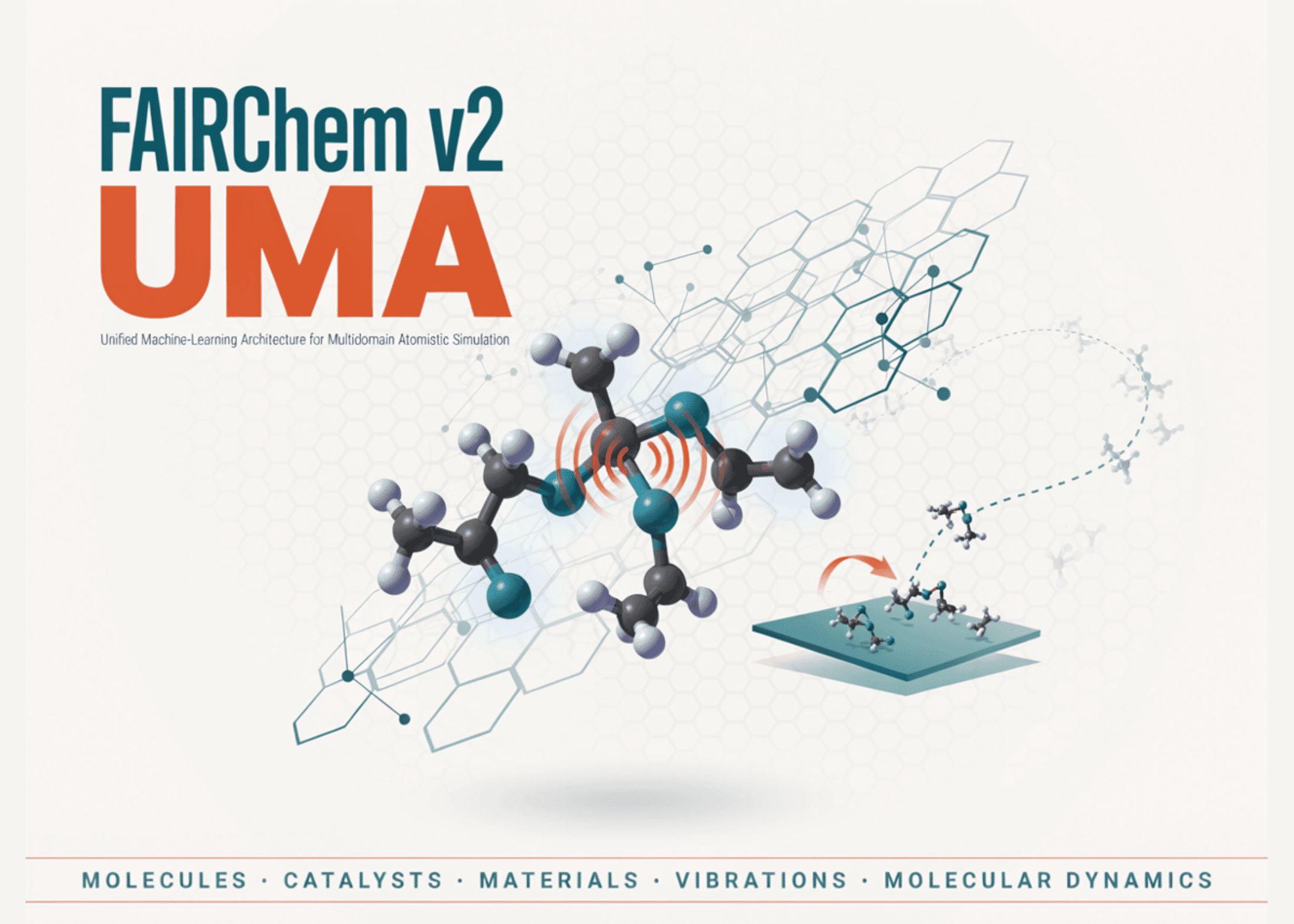
ในบทช่วยสอนนี้ เราจะเจาะลึกการใช้ FAIRChem v2 และศักย์ไฟฟ้าระหว่างอะตอมแบบแมชชีนเลิร์นนิงสากล UMA ในฐานะโครงร่างการทำงานแบบรวมศูนย์สำหรับการจำลองระดับอะตอมที่ครอบคลุมทั้งเคมีโมเลกุล การเร่งปฏิกิริยา และวัสดุอนินทรีย์ โดยเริ่มจากการกำหนดค่าสภาพแวดล้อม การรับรองความถูกต้องด้วย Hugging Face เพื่อเข้าถึงค่าน้ำหนักโมเดล UMA ที่มีการจำกัดสิทธิ์ ไปจนถึงการตั้งค่าตัวคำนวณ (calculators) เฉพาะงานสำหรับโดเมน omol, oc20 และ omat
เราจะนำศักย์ไฟฟ้าที่ผ่านการฝึกไว้ล่วงหน้า (pretrained potential) ชุดเดียวกันนี้ ไปประยุกต์ใช้กับเวิร์กโฟลว์เคมีคำนวณที่หลากหลาย เช่น การทำนายพลังงานและแรงแบบจุดเดียว (single-point energy and force prediction), การหาโครงสร้างโมเลกุลที่เหมาะสม (molecular geometry optimization), การวิเคราะห์การสั่นสะเทือน (vibrational analysis), การดูดซับที่พื้นผิว (surface adsorption) และพลศาสตร์โมเลกุล (molecular dynamics) โดยหัวใจสำคัญคือการผสาน FAIRChem เข้ากับ Atomic Simulation Environment (ASE) เพื่อจัดการโครงสร้างอะตอมและการคำนวณทางอุณหพลศาสตร์ พร้อมรองรับการเร่งความเร็วด้วย GPU
import importlib.util, subprocess, sys, os
def _pip(*pkgs):
    subprocess.check_call([sys.executable, "-m", "pip", "install", "-q", *pkgs])
if importlib.util.find_spec("fairchem") is None:
    print(">> Installing fairchem-core, ase, and helpers (takes ~2-4 min)...")
    _pip("fairchem-core", "ase", "matplotlib", "huggingface_hub")
    print(">> Installation done.")
else:
    print(">> fairchem already installed.")
from huggingface_hub import login, whoami
def hf_authenticate():
    token = None
    try:
        from google.colab import userdata
        token = userdata.get("HF_TOKEN")
    except Exception:
        pass
    token = token or os.environ.get("HF_TOKEN")
    try:
        whoami()
        print(">> Already authenticated with Hugging Face.")
        return
    except Exception:
        pass
    if token is None:
        from getpass import getpass
        token = getpass("Paste your Hugging Face access token: ").strip()
    login(token=token)
    print(">> Hugging Face login OK.")
hf_authenticate()
import numpy as np
import torch
import matplotlib.pyplot as plt
from fairchem.core import pretrained_mlip, FAIRChemCalculator
DEVICE = "cuda" if torch.cuda.is_available() else "cpu"
print(f">> Using device: {DEVICE}")
MODEL = "uma-s-1p2"
predictor = pretrained_mlip.get_predict_unit(MODEL, device=DEVICE)
calc_mol = FAIRChemCalculator(predictor, task_name="omol")
calc_cat = FAIRChemCalculator(predictor, task_name="oc20")
calc_mat = FAIRChemCalculator(predictor, task_name="omat")
print(f">> Loaded {MODEL} with omol / oc20 / omat calculators.")
กระบวนการเริ่มต้นด้วยการติดตั้งแพ็กเกจสำคัญอย่าง FAIRChem, ASE และเครื่องมือสร้างภาพต่างๆ โดยออกแบบให้สามารถรันบน Google Colab ได้อย่างปลอดภัย ระบบจะทำการยืนยันตัวตนกับ Hugging Face เพื่อดึงพารามิเตอร์ของโมเดล UMA และตรวจหาการใช้งาน GPU โดยอัตโนมัติ จากนั้นจึงสร้างตัวคำนวณแยกตามวัตถุประสงค์ ทั้งงานด้านโมเลกุล งานเร่งปฏิกิริยา และวัสดุศาสตร์
from ase.build import molecule
from ase import Atoms
print("\n" + "="*70)
print("SECTION 2: Single-point energetics of water (omol task)")
print("="*70)
h2o = molecule("H2O")
h2o.info.update({"charge": 0, "spin": 1})
h2o.calc = calc_mol
E_h2o = h2o.get_potential_energy()
F_h2o = h2o.get_forces()
print(f"E(H2O) = {E_h2o:.4f} eV")
print(f"Max |force| = {np.abs(F_h2o).max():.4f} eV/A")
def atom_energy(symbol, spin):
    a = Atoms(symbol, positions=[[0, 0, 0]])
    a.info.update({"charge": 0, "spin": spin})
    a.calc = calc_mol
    return a.get_potential_energy()
E_O = atom_energy("O", spin=3)
E_H = atom_energy("H", spin=2)
E_atomization = -(E_h2o - E_O - 2 * E_H)
print(f"Atomization energy of H2O = {E_atomization:.3f} eV "
      f"(experiment ~ 9.5 eV incl. ZPE effects)")
from ase.optimize import LBFGS
print("\n" + "="*70)
print("SECTION 3: Relaxing a deliberately distorted water molecule")
print("="*70)
h2o_bad = molecule("H2O")
h2o_bad.positions[1] += [0.25, -0.10, 0.05]
h2o_bad.info.update({"charge": 0, "spin": 1})
h2o_bad.calc = calc_mol
opt = LBFGS(h2o_bad, logfile=None)
energies_opt = []
opt.attach(lambda: energies_opt.append(h2o_bad.get_potential_energy()))
opt.run(fmax=0.01, steps=200)
d_OH = h2o_bad.get_distance(0, 1)
ang = h2o_bad.get_angle(1, 0, 2)
print(f"Converged in {opt.get_number_of_steps()} steps")
print(f"O-H bond length = {d_OH:.3f} A (expt ~0.958 A)")
print(f"H-O-H angle = {ang:.1f} deg (expt ~104.5 deg)")
plt.figure(figsize=(5, 3.2))
plt.plot(energies_opt, "o-")
plt.xlabel("Optimizer step"); plt.ylabel("Energy (eV)")
plt.title("H2O geometry optimization"); plt.tight_layout(); plt.show()
การสาธิตในส่วนแรกใช้ตัวคำนวณ UMA สำหรับโมเลกุลเพื่อวิเคราะห์พลังงาน แรง และพลังงานแตกตัว (atomization energy) ของน้ำ โดยกำหนดค่า spin multiplicities ของอะตอมไฮโดรเจนและออกซิเจนให้ถูกต้อง นอกจากนี้ยังทดลองทำให้โมเลกุลน้ำผิดรูปและใช้ตัวหาความเหมาะสม LBFGS เพื่อผ่อนคลายโครงสร้างกลับสู่จุดสมดุล พร้อมวิเคราะห์ความยาวและมุมพันธะเปรียบเทียบกับค่าจริงจากการทดลอง
print("\n" + "="*70)
print("SECTION 4: CH2 singlet-triplet gap (UMA is spin-aware!)")
print("="*70)
singlet = molecule("CH2_s1A1d"); singlet.info.update({"charge": 0, "spin": 1})
triplet = molecule("CH2_s3B1d"); triplet.info.update({"charge": 0, "spin": 3})
singlet.calc = FAIRChemCalculator(predictor, task_name="omol")
triplet.calc = FAIRChemCalculator(predictor, task_name="omol")
gap = triplet.get_potential_energy() - singlet.get_potential_energy()
print(f"E(triplet) - E(singlet) = {gap:.3f} eV "
      f"(negative => triplet ground state; expt ~ -0.39 eV)")
print("\n" + "="*70)
print("SECTION 5: Reaction energy of CH4 + 2 O2 -> CO2 + 2 H2O")
print("="*70)
def relaxed_energy(name, spin=1):
    m = molecule(name)
    m.info.update({"charge": 0, "spin": spin})
    m.calc = FAIRChemCalculator(predictor, task_name="omol")
    LBFGS(m, logfile=None).run(fmax=0.02, steps=200)
    return m.get_potential_energy()
E = {
    "CH4": relaxed_energy("CH4"),
    "O2": relaxed_energy("O2", spin=3),
    "CO2": relaxed_energy("CO2"),
    "H2O": relaxed_energy("H2O"),
}
dE_rxn = (E["CO2"] + 2*E["H2O"]) - (E["CH4"] + 2*E["O2"])
print(f"Delta E (electronic) = {dE_rxn:.2f} eV = {dE_rxn*96.485:.0f} kJ/mol")
print("Experimental combustion enthalpy ~ -890 kJ/mol (ZPE/thermal not included here)")
from ase.vibrations import Vibrations
print("\n" + "="*70)
print("SECTION 6: Vibrational frequencies of relaxed H2O")
print("="*70)
vib = Vibrations(h2o_bad, name="vib_h2o")
vib.run()
freqs = np.real(vib.get_frequencies())
real_modes = [f for f in freqs if f > 200]
print("Vibrational modes (cm^-1):", ", ".join(f"{f:.0f}" for f in real_modes))
print("Experimental H2O: 1595 (bend), 3657 (sym stretch), 3756 (asym stretch)")
print(f"Zero-point energy = {vib.get_zero_point_energy():.3f} eV")
vib.clean()
ส่วนถัดมาแสดงความสามารถในการรับรู้สถานะสปิน (spin-aware) ของ UMA ผ่านการคำนวณช่องว่างพลังงานระหว่างสถานะซิงเกลตและทริปเลตของเมทิลีน รวมถึงการประมาณค่าพลังงานปฏิกิริยาเผาไหม้ของมีเทน นอกจากนี้ยังมีการวิเคราะห์การสั่นสะเทือนเพื่อหาความถี่ในโหมดปกติและค่าพลังงานจุดศูนย์ (zero-point energy) ซึ่งเป็นค่าสำคัญในเคมีเชิงคำนวณ
from ase.build import fcc100, add_adsorbate
from ase.constraints import FixAtoms
print("\n" + "="*70)
print("SECTION 7: CO/Cu(100) relaxation + adsorption energy (oc20 task)")
print("="*70)
slab = fcc100("Cu", size=(3, 3, 3), vacuum=8.0, periodic=True)
slab.set_constraint(FixAtoms(mask=[a.tag > 1 for a in slab]))
add_adsorbate(slab, molecule("CO"), height=2.0, position="bridge")
slab.calc = calc_cat
opt = LBFGS(slab, logfile=None)
opt.run(fmax=0.05, steps=300)
E_slab_ads = slab.get_potential_energy()
print(f"Relaxed CO/Cu(100) in {opt.get_number_of_steps()} steps, "
      f"E = {E_slab_ads:.3f} eV")
clean = fcc100("Cu", size=(3, 3, 3), vacuum=8.0, periodic=True)
clean.set_constraint(FixAtoms(mask=[a.tag > 1 for a in clean]))
clean.calc = FAIRChemCalculator(predictor, task_name="oc20")
LBFGS(clean, logfile=None).run(fmax=0.05, steps=300)
E_clean = clean.get_potential_energy()
co = molecule("CO"); co.info.update({"charge": 0, "spin": 1})
co.calc = FAIRChemCalculator(predictor, task_name="omol")
LBFGS(co, logfile=None).run(fmax=0.02, steps=100)
E_co = co.get_potential_energy()
E_ads = E_slab_ads - E_clean - E_co
print(f"E(clean slab) = {E_clean:.3f} eV, E(CO gas) = {E_co:.3f} eV")
print(f"Adsorption energy (naive cycle) = {E_ads:.3f} eV")
print("(oc20 uses its own DFT reference scheme; for publication-grade numbers")
print(" keep all species within a consistent task/reference framework.)")
ในการประยุกต์ใช้กับตัวเร่งปฏิกิริยา เราได้สร้างแบบจำลองสแล็บของทองแดง Cu(100) และทดสอบการดูดซับของคาร์บอนมอนอกไซด์ โดยใช้ตัวคำนวณ OC20 เพื่อผ่อนคลายโครงสร้างพื้นผิว แม้ว่า OC20 จะมีวิธีอ้างอิงพลังงานเฉพาะตัว แต่โมเดลก็สามารถทำนายพลังงานการดูดซับเบื้องต้นออกมาได้อย่างน่าสนใจ
from ase.build import bulk
from ase.optimize import FIRE
from ase.filters import FrechetCellFilter
from ase.eos import EquationOfState
print("\n" + "="*70)
print("SECTION 8: BCC iron — full cell relaxation and bulk modulus (omat)")
print("="*70)
fe = bulk("Fe", "bcc", a=2.9)
fe.calc = calc_mat
FIRE(FrechetCellFilter(fe), logfile=None).run(fmax=0.02, steps=300)
a_relaxed = fe.cell.cellpar()[0]
print(f"Relaxed BCC Fe lattice constant = {a_relaxed:.3f} A (expt ~2.866 A)")
volumes, energies = [], []
cell0 = fe.get_cell()
for scale in np.linspace(0.94, 1.06, 9):
    s = fe.copy()
    s.set_cell(cell0 * scale, scale_atoms=True)
    s.calc = FAIRChemCalculator(predictor, task_name="omat")
    volumes.append(s.get_volume())
    energies.append(s.get_potential_energy())
eos = EquationOfState(volumes, energies, eos="birchmurnaghan")
v0, e0, B = eos.fit()
from ase.units import GPa as _GPa
B_GPa = B / _GPa
print(f"Equilibrium volume = {v0:.2f} A^3/cell")
print(f"Bulk modulus = {B_GPa:.0f} GPa (expt ~170 GPa for Fe)")
plt.figure(figsize=(5, 3.2))
plt.plot(volumes, energies, "o", label="UMA points")
vfit = np.linspace(min(volumes), max(volumes), 100)
plt.plot(vfit, [eos.func(v, *eos.eos_parameters) for v in vfit], "-", label="BM fit")
plt.xlabel("Volume (A^3)"); plt.ylabel("Energy (eV)")
plt.title("BCC Fe equation of state"); plt.legend(); plt.tight_layout(); plt.show()
from ase import units
from ase.md.langevin import Langevin
from ase.md.velocitydistribution import MaxwellBoltzmannDistribution
print("\n" + "="*70)
print("SECTION 9: 0.5 ps Langevin MD of a water molecule at 300 K")
print("="*70)
md_atoms = molecule("H2O")
md_atoms.info.update({"charge": 0, "spin": 1})
seed = int(np.random.randint(0, np.iinfo(np.int32).max))
md_predictor = pretrained_mlip.get_predict_unit(MODEL, device=DEVICE, seed=seed)
md_atoms.calc = FAIRChemCalculator(md_predictor, task_name="omol")
MaxwellBoltzmannDistribution(md_atoms, temperature_K=300)
dyn = Langevin(md_atoms, timestep=0.5 * units.fs,
               temperature_K=300, friction=0.01 / units.fs)
times, temps, epots, d_oh1 = [], [], [], []
def log_md():
    t = dyn.get_number_of_steps() * 0.5
    times.append(t)
    temps.append(md_atoms.get_temperature())
    epots.append(md_atoms.get_potential_energy())
    d_oh1.append(md_atoms.get_distance(0, 1))
dyn.attach(log_md, interval=5)
dyn.run(steps=1000)
print(f"MD done. <T> = {np.mean(temps[10:]):.0f} K, "
      f"<d(O-H)> = {np.mean(d_oh1):.3f} A")
fig, ax = plt.subplots(1, 3, figsize=(12, 3.2))
ax[0].plot(times, temps); ax[0].set_title("Temperature (K)")
ax[1].plot(times, epots); ax[1].set_title("Potential energy (eV)")
ax[2].plot(times, d_oh1); ax[2].set_title("O-H bond length (A)")
for a in ax: a.set_xlabel("time (fs)")
plt.tight_layout(); plt.show()
สำหรับการศึกษาวัสดุ เราได้ทดลองผ่อนคลายเซลล์ผลึกของเหล็ก BCC และหาค่าความเข้มแข็งของวัสดุ (bulk modulus) ผ่านสมการสถานะ Birch–Murnaghan และปิดท้ายด้วยการรันพลศาสตร์โมเลกุล (MD) แบบ Langevin เพื่อสังเกตพฤติกรรมของโมเลกุลน้ำภายใต้อุณหภูมิ 300 เคลวิน ซึ่งแสดงให้เห็นถึงการแกว่งของความยาวพันธะและพลังงานศักย์ตามช่วงเวลาจริง
print("\n" + "="*70)
print("SECTION 10: O-H bond stretch scan in water")
print("="*70)
distances = np.linspace(0.7, 2.5, 25)
pes = []
for d in distances:
    a = molecule("H2O")
    a.info.update({"charge": 0, "spin": 1})
    vec = a.positions[1] - a.positions[0]
    a.positions[1] = a.positions[0] + vec / np.linalg.norm(vec) * d
    a.calc = FAIRChemCalculator(predictor, task_name="omol")
    pes.append(a.get_potential_energy())
pes = np.array(pes) - min(pes)
plt.figure(figsize=(5.5, 3.4))
plt.plot(distances, pes, "o-")
plt.axvline(0.958, ls="--", c="gray", label="expt r_e")
plt.xlabel("O-H distance (A)"); plt.ylabel("Relative energy (eV)")
plt.title("O-H stretch PES from UMA"); plt.legend()
plt.tight_layout(); plt.show()
print("\n" + "="*70)
print("TUTORIAL COMPLETE!")
print("="*70)
print("""
Next steps to explore:
* Swap MODEL to "uma-m-1p1" for higher accuracy (needs more GPU memory).
* Try task_name="odac" with a MOF CIF, or "omc" for molecular crystals.
* Larger MD: fairchem supports multi-GPU inference via workers=N
(pip install fairchem-core[extras]).
* Docs: https://fair-chem.github.io/
""")
การสแกนพื้นผิวพลังงานศักย์ (PES) ของพันธะ O–H ช่วยให้เราเห็นโปรไฟล์การแตกตัวของโมเลกุลน้ำได้อย่างชัดเจน โดยสรุปแล้ว FAIRChem v2 และ UMA ช่วยให้นักวิจัยสามารถสร้างเวิร์กโฟลว์การจำลองระดับอะตอมที่สมบูรณ์และยืดหยุ่นได้ โดยไม่จำเป็นต้องสลับโมเลกุลไปมาสำหรับงานแต่ละประเภท ถือเป็นรากฐานสำคัญในการขยายผลสู่การศึกษาวัสดุที่ซับซ้อนยิ่งขึ้น เช่น โครงสร้างโลหะ-อินทรีย์ (MOF) หรือพื้นผิวตัวเร่งปฏิกิริยาในอนาคต
ดู ** Full Code ได้ที่นี่ ** นอกจากนี้ อย่าลังเลที่จะติดตามเราบน
ความคิดเห็น (0)
เข้าสู่ระบบเพื่อร่วมแสดงความเห็น
สมัครสมาชิกมาเป็นคนแรกที่แสดงความเห็นกันเลยโบร