
สร้าง Plasmid Engineering Workbench ด้วย Biopython และ Google Colab
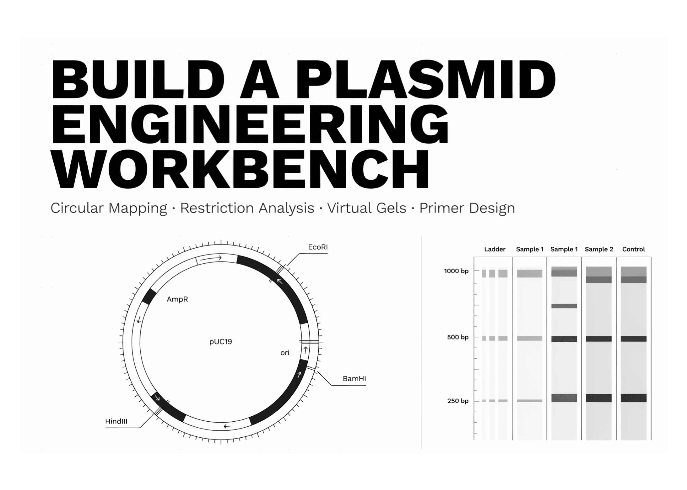
ในบทช่วยสอนนี้ เราจะสร้างเวิร์กเบนช์พลาสมิดบน Google Colab ที่จำลองแนวคิดหลักของ SpliceCraft ภายในสภาพแวดล้อมโน้ตบุ๊กแบบโต้ตอบ แทนที่จะใช้ TUI บนเทอร์มินัล เราจะเปลี่ยนมาใช้ Biopython, NumPy และ Matplotlib เพื่อโหลดข้อมูลเรคคอร์ดพลาสมิด, ปรับแต่งฟีเจอร์จีโนมิก, เรนเดอร์แผนที่พลาสมิดทั้งแบบวงกลมและเส้นตรง, คำนวณสถิติลำดับ, วิเคราะห์ตำแหน่งตัดของเอนไซม์จำเพาะ, จำลองการย่อยเสมือน (virtual digests), สแกนหา ORF (open reading frames), แปลรหัสฟีเจอร์ CDS, ออกแบบไพรม์เมอร์ และใช้โปรแกรมในการแก้ไขลำดับสายดีเอ็นเอ โดยเราจะเริ่มจากพลาสมิดสังเคราะห์แบบออฟไลน์เพื่อให้เวิร์กโฟลว์เสถียรที่สุด แต่ยังคงรองรับการดึงข้อมูลจาก NCBI GenBank หรือการอัปโหลดไฟล์ส่วนตัวได้ตามต้องการ
try:
    import Bio
except ImportError:
    import subprocess, sys
    subprocess.run([sys.executable, "-m", "pip", "install", "-q", "biopython"], check=True)
import math, io, textwrap, random
import numpy as np
import matplotlib
import matplotlib.pyplot as plt
from matplotlib.patches import Polygon
from Bio import Entrez, SeqIO
from Bio.Seq import Seq
from Bio.SeqRecord import SeqRecord
from Bio.SeqFeature import SeqFeature, FeatureLocation
from Bio.Restriction import RestrictionBatch, Analysis, CommOnly
try:
    from Bio.SeqUtils import MeltingTemp as _mt
except Exception:
    _mt = None
EMAIL = "[[email protected]](https://www.marktechpost.com/cdn-cgi/l/email-protection)"
ACCESSION = "L09137"
USE_NCBI = False
Entrez.email = EMAIL
TYPE_COLORS = {
    "CDS": "#d1495b", "gene": "#c1666b", "rep_origin": "#2e86ab",
    "promoter": "#e3a008", "terminator": "#8d99ae", "misc_feature": "#6a994e",
    "primer_bind": "#9d4edd", "protein_bind": "#457b9d", "source": "#adb5bd",
}
def _color(ftype): return TYPE_COLORS.get(ftype, "#6a994e")
MCS = "GAATTCGAGCTCGGTACCCGGGGATCCTCTAGAGTCGACCTGCAGGCATGCAAGCTT"
def _synthetic_plasmid():
    random.seed(19)
    body = "".join(random.choice("ACGT") for _ in range(2686))
    seq = body[:400] + MCS + body[400:]
    rec = SeqRecord(Seq(seq), id="pDEMO", name="pDEMO",
                    description="Synthetic offline demo plasmid (SpliceCraft-Colab)")
    rec.annotations["topology"] = "circular"
    rec.annotations["molecule_type"] = "ds-DNA"
    def feat(s, e, strand, ftype, label):
        f = SeqFeature(FeatureLocation(s, e, strand=strand), type=ftype)
        f.qualifiers["label"] = [label]; return f
    rec.features += [
        feat(400, 400 + len(MCS), 1, "misc_feature", "MCS"),
        feat(700, 1561, 1, "CDS", "AmpR"),
        feat(1700, 2260, -1, "rep_origin", "ori"),
        feat(2350, 2686, 1, "CDS", "lacZ-alpha"),
    ]
    rec.features[1].qualifiers["product"] = ["beta-lactamase (demo)"]
    return rec
def load_record():
    if USE_NCBI and "@" in EMAIL and not EMAIL.startswith("you@"):
        try:
            h = Entrez.efetch(db="nucleotide", id=ACCESSION,
                              rettype="gbwithparts", retmode="text")
            rec = SeqIO.read(h, "genbank"); h.close()
            print(f"✓ Fetched {ACCESSION} from NCBI: {rec.description}")
            return rec
        except Exception as e:
            print(f"⚠ NCBI fetch failed ({e}); using synthetic demo plasmid.")
    else:
        print("ℹ USE_NCBI is off (or EMAIL not set) — using synthetic demo plasmid.")
    return _synthetic_plasmid()
def upload_gb():
    from google.colab import files
    up = files.upload()
    name = next(iter(up))
    return SeqIO.read(io.StringIO(up[name].decode()), "genbank")
def label_of(f):
    for k in ("label", "gene", "product", "note"):
        if k in f.qualifiers: return f.qualifiers[k][0]
    return f.type
def norm_features(rec, skip_source=True, min_len=0):
    L = len(rec.seq); out = []
    for f in rec.features:
        if skip_source and f.type in ("source",): continue
        s = int(f.location.start); e = int(f.location.end)
        if (e - s) < min_len: continue
        out.append(dict(start=s % L, end=e % L, strand=f.location.strand or 1,
                        type=f.type, label=label_of(f), color=_color(f.type)))
    return out
ขั้นตอนแรกเริ่มจากการเตรียมสภาวะแวดล้อมบนโน้ตบุ๊ก ติดตั้ง Biopython และนำเข้าไลบรารีสำหรับการคำนวณและการพลอตกราฟ เราได้กำหนดค่าเริ่มต้นของพลาสมิด พิกัดตำแหน่งการโคลน (MCS) และจานสีสำหรับแต่ละฟีเจอร์ นอกจากนี้ยังมีฟังก์ชันเสริมในการโหลดข้อมูลจาก NCBI หรืออัปโหลดไฟล์ GenBank โดยตรง พร้อมแปลงข้อมูลจีโนมิกให้พร้อมสำหรับการแสดงผล
def _ang(bp, L): return math.pi/2 - 2*math.pi*(bp/L)
def _pt(bp, r, L):
    a = _ang(bp, L); return r*math.cos(a), r*math.sin(a)
def _arc(s, e, r, L, n=240):
    if e < s: e += L
    bps = np.linspace(s, e, max(2, int(n*(e-s)/L)+2))
    return ([r*math.cos(_ang(b, L)) for b in bps],
            [r*math.sin(_ang(b, L)) for b in bps])
def gc_percent(seq):
    s = str(seq).upper(); n = len(s) or 1
    return 100.0 * (s.count("G") + s.count("C")) / n
def circular_map(rec, title=None, show_gc=True):
    L = len(rec.seq); feats = norm_features(rec)
    fig, ax = plt.subplots(figsize=(8, 8)); R = 1.0
    if show_gc:
        w = max(30, L // 120); step = max(1, w // 2); mean = gc_percent(rec.seq)
        s = str(rec.seq).upper()
        for i in range(0, L, step):
            win = s[i:i+w] or s[i:] + s[:(i+w) % L]
            dev = (gc_percent(win) - mean) / 100.0
            rr = 0.72 + dev * 0.9
            x0, y0 = _pt(i, 0.72, L); x1, y1 = _pt(i, rr, L)
            ax.plot([x0, x1], [y0, y1],
                    color="#2e86ab" if dev >= 0 else "#d1495b", lw=1, alpha=0.5, zorder=1)
    xs, ys = _arc(0, L, R, L); ax.plot(xs, ys, color="#333", lw=2.5, zorder=2)
    step = max(1, round(L/12/100)*100) or max(1, L//12)
    for t in range(0, L, step):
        x0, y0 = _pt(t, R*1.015, L); x1, y1 = _pt(t, R*1.045, L)
        ax.plot([x0, x1], [y0, y1], color="#999", lw=1, zorder=2)
        lx, ly = _pt(t, R*1.10, L)
        ax.text(lx, ly, f"{t:,}", ha="center", va="center", fontsize=7, color="#777")
    for f in feats:
        outer = f["strand"] >= 0
        rr = R + 0.09 if outer else R - 0.09
        xs, ys = _arc(f["start"], f["end"], rr, L)
        ax.plot(xs, ys, color=f["color"], lw=10, solid_capstyle="butt", alpha=0.9, zorder=3)
        tip = f["end"] if outer else f["start"]
        a = _ang(tip, L); tx, ty = rr*math.cos(a), rr*math.sin(a)
        d = -1 if outer else 1
        tanx, tany = -math.sin(a)*d, math.cos(a)*d
        px, py = math.cos(a), math.sin(a)
        ln, wd = 0.055, 0.052
        ax.add_patch(Polygon([(tx+tanx*ln, ty+tany*ln),
                              (tx+px*wd, ty+py*wd),
                              (tx-px*wd, ty-py*wd)],
                             color=f["color"], zorder=4))
        span = (f["end"] - f["start"]) % L
        mid = (f["start"] + span/2) % L
        lx, ly = _pt(mid, (rr + 0.16) if outer else (rr - 0.16), L)
        ax.text(lx, ly, f["label"], ha="center", va="center",
                fontsize=8.5, color=f["color"], weight="bold", zorder=5)
    circ = "circular" if rec.annotations.get("topology") == "circular" else "linear"
    ax.text(0, 0.05, title or rec.name, ha="center", va="center", fontsize=15, weight="bold")
    ax.text(0, -0.07, f"{L:,} bp · {gc_percent(rec.seq):.1f}% GC · {circ}",
            ha="center", va="center", fontsize=9.5, color="#555")
    ax.set_xlim(-1.45, 1.45); ax.set_ylim(-1.45, 1.45)
    ax.set_aspect("equal"); ax.axis("off"); plt.tight_layout(); plt.show()
สำหรับการแสดงผลแผนที่แบบวงกลม เราใช้การแปลพิกัดจากคู่เบสเป็นมุมองศาบนวงกลมตามเข็มนาฬิกา โดยสามารถแสดงเนื้อหา GC, โครงสร้างหลักของพลาสมิด (Backbone), มาตราส่วน และทิศทางของยีนด้วยหัวลูกศร (Strand orientation) อย่างแม่นยำ พร้อมระบุเมตาเดตาสำคัญไว้ตรงกลางเพื่อให้แผนที่อ่านง่ายและได้ข้อมูลครบถ้วน
def linear_map(rec):
    L = len(rec.seq); feats = norm_features(rec)
    fig, ax = plt.subplots(figsize=(11, 2.6))
    ax.hlines(0, 0, L, color="#333", lw=2)
    for f in feats:
        y = 0.35 if f["strand"] >= 0 else -0.35
        s, e = f["start"], f["end"]
        segs = [(s, e)] if e >= s else [(s, L), (0, e)]
        for a, b in segs:
            ax.annotate("", xy=(b if f["strand"] >= 0 else a, y),
                        xytext=(a if f["strand"] >= 0 else b, y),
                        arrowprops=dict(arrowstyle="-|>", color=f["color"], lw=7, alpha=0.85))
        ax.text((s + ((e - s) % L)/2) % L, y + (0.28 if y > 0 else -0.28), f["label"],
                ha="center", va="center", fontsize=8.5, color=f["color"], weight="bold")
    ax.set_xlim(-L*0.02, L*1.02); ax.set_ylim(-1, 1)
    ax.set_yticks([]); ax.set_xlabel("position (bp)")
    ax.set_title(f"{rec.name} — linear view", fontsize=11)
    for sp in ("top", "left", "right"): ax.spines[sp].set_visible(False)
    plt.tight_layout(); plt.show()
def gc_skew_plot(rec, window=None):
    s = str(rec.seq).upper(); L = len(s)
    window = window or max(50, L // 100); skew = []; run = 0
    for i in range(0, L, window):
        w = s[i:i+window]; g, c = w.count("G"), w.count("C")
        run += (g - c) / max(1, g + c); skew.append(run)
    fig, ax = plt.subplots(figsize=(11, 2.6))
    ax.plot(np.arange(len(skew))*window, skew, color="#2e86ab")
    ax.axhline(0, color="#aaa", lw=0.8)
    ax.set_title(f"Cumulative GC-skew — {rec.name} (min≈replication origin, max≈terminus)",
                 fontsize=10)
    ax.set_xlabel("position (bp)"); ax.set_ylabel("cumulative skew")
    plt.tight_layout(); plt.show()
def stats(rec):
    seq = str(rec.seq).upper(); L = len(seq)
    print(f"── {rec.name} ─────────────────────────────")
    print(f"length   : {L:,} bp")
    print(f"GC content : {gc_percent(seq):.2f} %")
    print(f"A/T/G/C  : {seq.count('A')}/{seq.count('T')}/{seq.count('G')}/{seq.count('C')}")
    print(f"topology : {rec.annotations.get('topology', 'unknown')}")
    print(f"features : {len(norm_features(rec))} annotated")
def _is_circular(rec): return rec.annotations.get("topology") == "circular"
def find_sites(rec, enzymes=None):
    batch = RestrictionBatch(enzymes) if enzymes else CommOnly
    ana = Analysis(batch, rec.seq, linear=not _is_circular(rec))
    return {str(k): v for k, v in ana.full().items()}
def unique_cutters(rec, enzymes=None):
    hits = find_sites(rec, enzymes)
    return sorted([e for e, pos in hits.items() if len(pos) == 1])
def digest_fragments(rec, enzymes):
    hits = find_sites(rec, enzymes)
    cuts = sorted({p for pos in hits.values() for p in pos})
    L = len(rec.seq)
    if not cuts: return [L]
    if _is_circular(rec):
        frags = [cuts[i+1] - cuts[i] for i in range(len(cuts)-1)]
        frags.append(L - cuts[-1] + cuts[0])
    else:
        frags = [cuts[0]] + [cuts[i+1]-cuts[i] for i in range(len(cuts)-1)] + [L - cuts[-1]]
    return sorted((f for f in frags if f > 0), reverse=True)
def restriction_report(rec, enzymes=None):
    hits = find_sites(rec, enzymes)
    cutting = {e: p for e, p in hits.items() if p}
    print(f"── Restriction map of {rec.name} "
          f"({'circular' if _is_circular(rec) else 'linear'}) ──")
    print(f"unique (single) cutters: {', '.join(unique_cutters(rec, enzymes)) or 'none'}")
    print("cutting enzymes (site count):")
    for e in sorted(cutting, key=lambda x: len(cutting[x])):
        print(f"  {e:<10} {len(cutting[e])}x at {cutting[e]}")
เราพัฒนายูทิลิตี้เพิ่มเติมเพื่อสร้างแผนที่แบบเส้นตรงสำหรับการตรวจสอบพิกัดที่ละเอียดขึ้น พร้อมคำนวณค่า GC-skew สะสมเพื่อหาตำแหน่งต้นกำเนิดการจำลองตัว (Replication origin) นอกจากนี้ยังมีระบบวิเคราะห์การตัดจำเพาะ (Restriction analysis) เพื่อระบุตำแหน่งตัดของเอนไซม์และประเมินขนาดชิ้นส่วนดีเอ็นเอที่ได้จากการย่อย
def virtual_gel(named_digests):
    lanes = [("Ladder", LADDER)] + list(named_digests.items())
    fig, ax = plt.subplots(figsize=(1.4*len(lanes)+1, 6))
    ax.set_facecolor("#0b1021")
    def y(sz): return math.log10(max(sz, 50))
    for i, (name, frags) in enumerate(lanes):
        for f in frags:
            ax.hlines(y(f), i+0.62, i+1.38, color="#e6f1ff",
                      lw=2 + min(4, f/1500), alpha=0.9)
        if name == "Ladder":
            ax.text(i+0.5, y(f), f"{f}", color="#9db4d0", ha="right",
                    va="center", fontsize=7)
        ax.text(i+1, y(max(LADDER))+0.15, name, color="#e6f1ff",
                ha="center", fontsize=9, rotation=0)
    ax.set_xlim(0.2, len(lanes)+0.5); ax.set_ylim(y(80), y(12000))
    ax.invert_yaxis(); ax.axis("off")
    ax.set_title("Virtual agarose gel", color="#333", fontsize=11)
    plt.tight_layout(); plt.show()
def find_orfs(rec, min_aa=50):
    seq = rec.seq; L = len(seq); orfs = []
    for strand, s in ((+1, seq), (-1, seq.reverse_complement())):
        s = str(s)
        for frame in range(3):
            i = frame
            while i < L - 2:
                if s[i:i+3] == "ATG":
                    j = i
                    while j < L - 2:
                        if s[j:j+3] in ("TAA", "TAG", "TGA"):
                            if (j - i)//3 >= min_aa:
                                orfs.append((strand, frame, i, j+3, (j-i)//3))
                            i = j; break
                        j += 3
                i += 3
    return sorted(orfs, key=lambda o: -o[4])
def translate_feature(rec, label):
    for f in rec.features:
        if label.lower() in label_of(f).lower() and f.type in ("CDS", "gene"):
            sub = f.location.extract(rec.seq)
            prot = sub.translate(table=11, to_stop=True)
            return str(prot)
    return None
def _tm(primer):
    if _mt is not None:
        try: return float(_mt.Tm_NN(Seq(primer)))
        except Exception: pass
    p = primer.upper()
    return 2*(p.count('A')+p.count('T')) + 4*(p.count('G')+p.count('C'))
def design_primers(rec, start, end, target_tm=60.0, lo=18, hi=30):
    seq = str(rec.seq)
    def tune(sub, rev=False):
        best = None
        for n in range(lo, hi+1):
            p = sub[-n:] if rev else sub[:n]
            if rev: p = str(Seq(p).reverse_complement())
            score = abs(_tm(p) - target_tm)
            if best is None or score < best[0]: best = (score, p)
        return best[1]
    fwd = tune(seq[start:start+hi])
    rev = tune(seq[end-hi:end], rev=True)
    print(f"── Primers to amplify {start}–{end} ({end-start} bp) ──")
    print(f" FWD 5'-{fwd}-3' len {len(fwd)} Tm {_tm(fwd):.1f}°C GC {gc_percent(fwd):.0f}%")
    print(f" REV 5'-{rev}-3' len {len(rev)} Tm {_tm(rev):.1f}°C GC {gc_percent(rev):.0f}%")
    print(f" amplicon: {end-start} bp")
    return fwd, rev
จุดเด่นของเวิร์กเบนช์นี้คือระบบรันเจลอะกาโรสเสมือน (Virtual Gel) ที่แสดงผลบนสเกลลอการิทึมเทียบกับ DNA ladder นอกจากนี้ยังสามารถสแกนหา ORF ทั้ง 6 เฟรม, แปลรหัสพันธุกรรมจากโปรตีนในส่วน CDS และออกแบบไพรม์เมอร์โดยปรับแต่งค่าความยาวให้อุณหภูมิหลอมตัว (Tm) เข้าใกล้เป้าหมายมากที่สุด
def edit_sequence(rec, pos, delete=0, insert=""):
    s = str(rec.seq)
    new = s[:pos] + insert + s[pos+delete:]
    out = SeqRecord(Seq(new), id=rec.id, name=rec.name + "_edit",
                    description=rec.description + f" [edit @{pos}:-{delete}+{len(insert)}]")
    out.annotations = dict(rec.annotations)
    shift = len(insert) - delete
    for f in rec.features:
        s0, e0 = int(f.location.start), int(f.location.end)
        if s0 >= pos: s0 += shift
        if e0 > pos: e0 += shift
        if 0 <= s0 < e0 <= len(new):
            g = SeqFeature(FeatureLocation(s0, e0, strand=f.location.strand), type=f.type)
            g.qualifiers = dict(f.qualifiers); out.features.append(g)
    return out
LIBRARY = {}
def add_to_library(rec): LIBRARY[rec.name] = rec; print(f"+ added {rec.name} (now {len(LIBRARY)} in library)")
def show_library():
    for name, r in LIBRARY.items():
        print(f"  {name:<16} {len(r.seq):>7,} bp {gc_percent(r.seq):.1f}% GC")
ระบบยังรองรับการจัดการลำดับดีเอ็นเอ ไม่ว่าจะเป็นการแทรก ลบ หรือแทนที่ โดยยังคงรักษาข้อมูลประกอบ (Annotations) ของฟีเจอร์ต่างๆ ให้ขยับตามตำแหน่งที่แก้ไขจริง พร้อมระบบไลบรารีขนาดเล็กเพื่อจัดเก็บและเรียกใช้งานพลาสมิดหลายรุ่นพร้อมกัน
if __name__ == "__main__":
    rec = load_record()
    add_to_library(rec)
    print("\n[1] Sequence statistics")
    stats(rec)
    print("\n[2] Circular map (the signature SpliceCraft view)")
    circular_map(rec)
    print("\n[3] Linear map + GC-skew")
    linear_map(rec)
    gc_skew_plot(rec)
    print("\n[4] Restriction analysis")
    restriction_report(rec, enzymes=["EcoRI", "BamHI", "HindIII", "PstI",
                                     "SalI", "XbaI", "KpnI", "SacI", "SphI"])
    print("\n[5] Virtual digests on a gel")
    virtual_gel({
        "EcoRI": digest_fragments(rec, ["EcoRI"]),
        "EcoRI+HindIII": digest_fragments(rec, ["EcoRI", "HindIII"]),
        "BamHI+SalI": digest_fragments(rec, ["BamHI", "SalI"]),
    })
    print("\n[6] Six-frame ORF scan (top 5 by length)")
    for strand, frame, s, e, aa in find_orfs(rec, min_aa=40)[:5]:
        print(f" strand {strand:+d} frame {frame} {s}-{e} {aa} aa")
    print("\n[7] Translate a CDS feature")
    prot = translate_feature(rec, "AmpR")
    if prot: print(f" AmpR protein ({len(prot)} aa): {prot[:60]}...")
    print("\n[8] Design primers to amplify a region")
    design_primers(rec, 400, 900)
    print("\n[9] Edit the sequence (insert a 6-bp tag) and re-map")
    edited = edit_sequence(rec, pos=456, insert="CATCATCAT")
    add_to_library(edited)
    print("\n[10] Library"); show_library()
    print("\nDone. Call any function directly, e.g. circular_map(edited).")
การสาธิตแบบเต็มรูปแบบแสดงให้เห็นถึงเวิร์กโฟลว์ตั้งแต่ต้นจนจบ ตั้งแต่การวิเคราะห์สถิติไปจนถึงการแก้ไขลำดับและออกแบบไพรม์เมอร์ บทช่วยสอนนี้พิสูจน์ให้เห็นว่าเราสามารถเปลี่ยนโน้ตบุ๊กเพียงเครื่องเดียวให้กลายเป็นเครื่องมือชีวสารสนเทศที่มีประสิทธิภาพ ทำงานได้ซ้ำ และแสดงผลกราฟิกที่สวยงาม โดยสรุป เราได้สร้างพื้นที่ทำงานวิศวกรรมพลาสมิดที่ครบวงจรบน Google Colab ซึ่งช่วยให้การตรวจสอบเรคคอร์ด GenBank การปรับปรุงลำดับ และการเปรียบเทียบโครงสร้างที่แก้ไขแล้วทำได้สะดวกและยืดหยุ่นมากขึ้นผ่านการเขียนโปรแกรม Python
ตรวจสอบ ** FULL CODES ที่นี่ ** นอกจากนี้ โปรดติดตามเราบน
ความคิดเห็น (0)
เข้าสู่ระบบเพื่อร่วมแสดงความเห็น
สมัครสมาชิกมาเป็นคนแรกที่แสดงความเห็นกันเลยโบร