
เจาะลึกการทำ Profiling ใน PyTorch (ตอนที่ 3): วิเคราะห์ประสิทธิภาพ Attention แต่ละรูปแบบ
นี่คือโพสต์ที่สามของซีรีส์ Profiling ใน PyTorch ซึ่งเป็นซีรีส์ที่เราจะค่อยๆ เสริมสร้างทักษะการอ่าน profiler traces และนำไปใช้ในการทำ optimization:
- Profiling in PyTorch (Part 1): A Beginner's Guide to torch.profiler
- Profiling in PyTorch (Part 2): From nn.Linear to a Fused MLP
- Profiling in PyTorch (Part 3): Attention is all you profile (ตอนปัจจุบัน)
ซีรีส์ "Profiling in PyTorch" มีวัตถุประสงค์เพื่อให้คุณคุ้นเคยกับการอ่าน profiler traces และตารางต่างๆ ใน ตอนที่ 1 เราได้ทำ profiling การคำนวณพื้นฐานอย่างการบวกและการคูณ เราได้เห็นว่าตารางของ profiler เผยให้เห็นจุดที่มีการทำงานหนัก (hotspots) อย่างไร และ profiler trace แสดงลำดับการทำงานของอัลกอริทึมตามช่วงเวลาอย่างไร
ใน ตอนที่ 2 เราได้นำการบวกและการคูณเหล่านั้นมาห่อหุ้มใน torch linear layer จากนั้นเราได้วางซ้อน linear layer หลายชั้น (multilayer perceptron) และทำ profiling การทำงานนั้น นอกจากนี้เรายังได้ทำ profiling ตัว kernels แบบ fused และแบบที่ปรับแต่งด้วยมือ (hand-tuned)
จากมุมมองของสถาปัตยกรรม Transformer ขั้นตอนถัดไปที่สมเหตุสมผลสำหรับเราในการทำ profiling คืออีกหนึ่งอัลกอริทึมพื้นฐาน นั่นคือ attention แม้ว่ามันจะมีชื่อเสียเรื่องความซับซ้อนของเวลาในระดับกำลังสอง (quadratic-time complexity) แต่ก็มีเทคนิคที่ชาญฉลาดมากมายที่ช่วยบรรเทาปัญหานั้นและทำให้มันทำงานได้เร็วขึ้น เป้าหมายของเราที่นี่ไม่ใช่การลงรายละเอียดในทุกเทคนิค แต่เราต้องการดูว่าแต่ละเทคนิคมีลักษณะที่แตกต่างกันอย่างไรภายใต้ profiler
สคริปต์สำหรับบล็อกโพสต์นี้อยู่ที่นี่:
04_a_naive_attention.py,04_b_inplace_ops_attention.py,04_c_sdpa_attention.py, และ04_d_kernels_attention.pyเช่นเคย การเปิดสคริปต์เหล่านี้ในแท็บแยกต่างหากและไล่ดูโค้ดตามที่อ่านจะช่วยให้เข้าใจง่ายขึ้น เราใช้ GPUNVIDIA A100-SXM4-80GBในการรันสคริปต์ ซึ่งการตั้งค่า GPU บนโครงสร้างพื้นฐานของ Hugging Face นั้นทำได้ง่ายมาก และสามารถทดลองกับสคริปต์ได้โดยใช้ Dev Mode with Spaces หรือจะรันสคริปต์ด้วย Hugging Face Jobs pipeline ก็ได้เช่นกัน
Naive attention
Attention ทำงานร่วมกับ Queries (q), Keys (k), และ Values (v) โดยมีลำดับขั้นตอนสั้นๆ ดังนี้:
- สร้างคะแนน attention (
scores):matmul(q, k.T) - ปรับขนาดคะแนน (Scale):
scores * scale - ใช้ causal mask กับคะแนน:
scores.masked_fill(mask, "-inf") - ปรับคะแนนให้เป็นค่าปกติ (Normalize) ด้วย softmax เพื่อให้ได้ค่าน้ำหนัก attention (
attn):softmax(scores) - คำนวณค่าน้ำหนักใหม่ให้กับ values:
matmul(attn, v)
ดังนั้น attention จึงเป็นการรวมกลุ่มของ operations พื้นฐาน ลองเขียนโมดูล naive attention ใน PyTorch และทำ profiling กัน
class NaiveCausalAttention(nn.Module):
    def __init__(self, head_dim):
        super().__init__()
        self.scale = 1.0 / math.sqrt(head_dim)

def forward(self, q, k, v, mask):
        scores = torch.matmul(q, k.transpose(-2, -1))
        scores = scores * self.scale
        scores = scores.masked_fill(mask, float("-inf"))
        attn = torch.softmax(scores, dim=-1)
        out = torch.matmul(attn, v)
        return out
ก่อนเปิดดู trace เราคาดเดาว่าจะพบ:
- kernel สำหรับ matmul (
q . k.T) - kernel สำหรับ mul (การ scaling)
- operation สำหรับการ masking
- kernel สำหรับ softmax
- kernel สำหรับ matmul (
atten . v)
uv run 04_a_naive_attention.py
uvx trace-util -f traces/ -b <hf_uname>/traces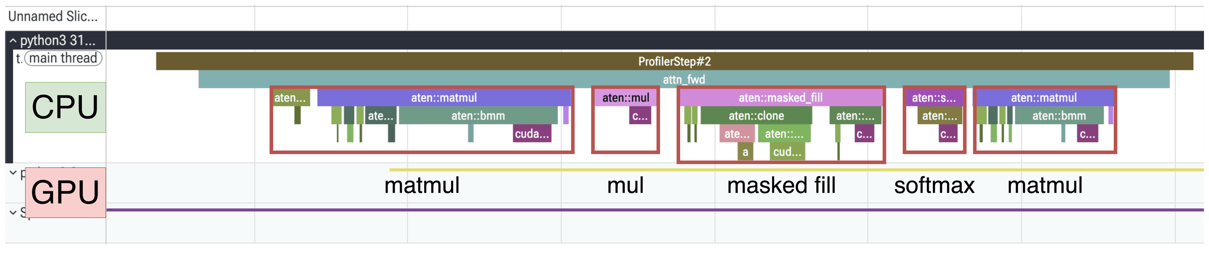 |
|---|
| รูปที่ 1: เลน CPU ของ profile trace สำหรับ naive attention ที่แสดง operations แยกส่วนกัน |
รูปที่ 1 แสดงผลลัพธ์ที่ตรงตามการคาดการณ์ของเราเป๊ะๆ ภายในบล็อก attn_fwd มีทั้ง matmul, mul (scaling), masked_fill และ softmax
คราวนี้ลองขยายเลน GPU เพื่อดู kernels ที่ถูกเรียกใช้งานจริง
 |
|---|
| รูปที่ 2: เลน GPU และ CPU ของ profile trace สำหรับ naive attention |
 |
|---|
| รูปที่ 3: ภาพขยายเลน GPU ของ naive attention |
รูปที่ 3 เผยให้เห็นสิ่งที่น่าสนใจคือมีการทำงาน 6 ขั้นตอน โดยมีขั้นตอนที่ 3 คือ memory copy โผล่มาอย่างแปลกแยก ซึ่งเกิดขึ้นเพราะการใช้ masked_fill แบบปกติ (out-of-place) ทำให้ PyTorch ต้องสำเนาข้อมูลก่อนดำเนินการ
Naive attention พร้อมการทำ inplace causal masking
เราจะลองเปลี่ยน masked_fill เป็นแบบ in-place โดยเติมเครื่องหมายขีดล่าง (_) เป็น masked_fill_ เพื่อลดการสำเนาข้อมูล
    def forward(self, q, k, v, mask):
        # ... เหมือนเดิม
-       scores = scores.masked_fill(mask, float("-inf"))
+       scores.masked_fill_(mask, float("-inf"))
        # ... เหมือนเดิม
uv run 04_b_inplace_ops_attention.py
uvx trace-util -f traces/ -b <hf_uname>/traces| ประเภท | CPU stream |
|---|---|
| รูปที่ 4: Naive masking | |
| รูปที่ 5: In place masking |  |
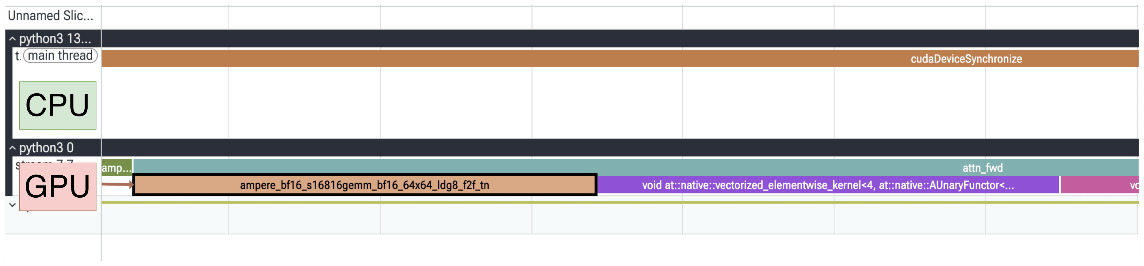
บนเลน GPU kernel Memcpy หายไปเรียบร้อยแล้ว (รูปที่ 6 และ 7) แม้จะดูเป็นจุดเล็กๆ แต่ในโมดูลขนาดใหญ่ที่มีหลายชั้น การประหยัดนี้จะส่งผลอย่างมาก
| ประเภท | GPU stream |
|---|---|
| รูปที่ 6: Naive masking | |
| รูปที่ 7: In place masking |  |
หมายเหตุ: การใช้ in-place ต้องระวังเรื่อง autograd แต่ในกรณีของ
forwardภายใต้torch.no_gradนั้นถือว่าปลอดภัยและช่วยประหยัดหน่วยความจำได้ดี
Scaled Dot Product Attention
ทีม PyTorch ได้รวมขั้นตอนทั้งหมดไว้ในฟังก์ชันเดียวคือ F.scaled_dot_product_attention (SDPA) ซึ่งมีการเลือก backend ที่เหมาะสมให้อัตโนมัติ
from torch.nn import functional as F
F.scaled_dot_product_attention(q, k, v, is_causal=True)
Math backend
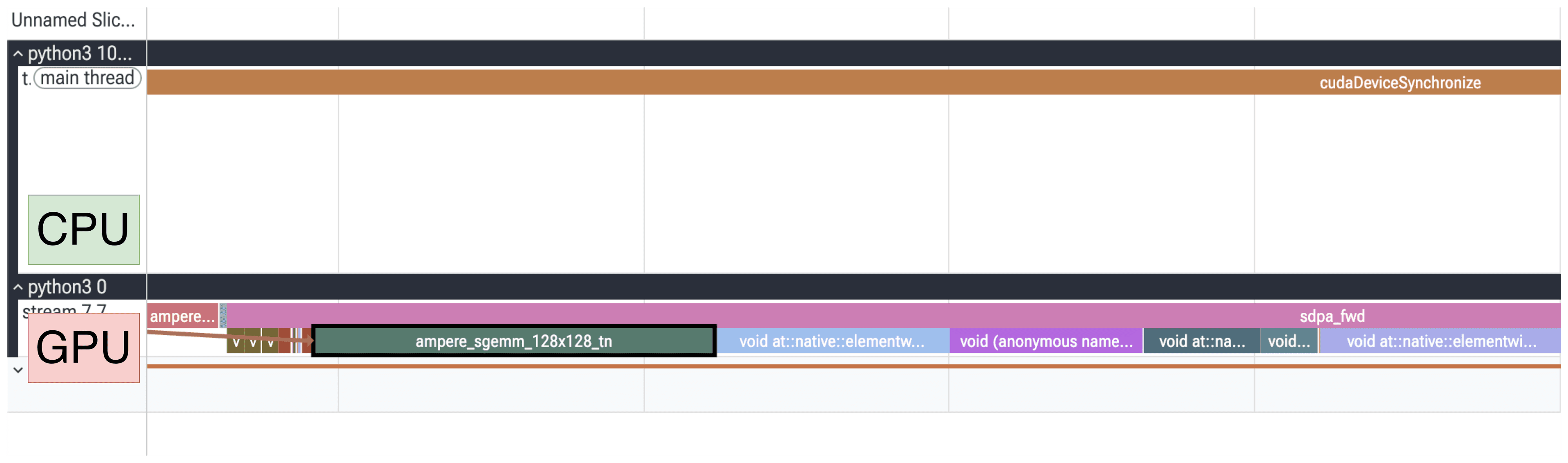
เมื่อบังคับใช้ math backend ผลลัพธ์กลับกลายเป็นว่าช้าลงถึง 3.7 เท่า และเรียกใช้ GPU kernels ถึง 20 ตัว
| Metric | Naive in-place | SDPA math |
|---|---|---|
*_fwd CUDA time avg | 1.955 ms | 7.239 ms |
| Self CUDA time total | 7.194 ms | 27.279 ms |
สาเหตุที่ช้าลง (ดูรูปที่ 8-13) เกิดจาก:
- ไม่ใช้ Tensor Cores: ตรวจพบรอยเซ็น
sgemmซึ่งรันบน CUDA cores แทนที่จะเป็นs16816บน Tensor Cores - การสร้าง Mask ใหม่: มีการสร้าง mask ใหม่จากศูนย์ในทุกรอบการเรียก
- Safe Softmax: ใช้
_safe_softmaxเพื่อป้องกัน NaN ซึ่งเพิ่มขั้นตอนการทำงาน โดยรวมแล้ว Math backend มีไว้เพื่อความถูกต้องแม่นยำและการรองรับที่ครอบคลุม (Reference Implementation) ไม่ได้เน้นความเร็วสูงสุด
Efficient backend
ใช้เทคนิคจากไลบรารี xformers โดยเรียกใช้ fused kernel เพียงตัวเดียวคือ fmha_cutlassF ซึ่งทำงานบน Tensor cores ด้วยรูปแบบ bfloat16 (รูปที่ 14)
Flash backend
ใช้ FlashAttention-2 ของ Tri Dao ซึ่งเน้นการลดภาระการรับส่งข้อมูลกับหน่วยความจำหลัก (HBM) โดยการคำนวณแบบ Tile และรักษาสถานะแบบ Online Softmax
 |
|---|
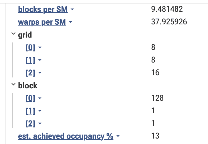
| รูปที่ 16: Flash kernel รายงานค่า occupancy เพียง 13% |
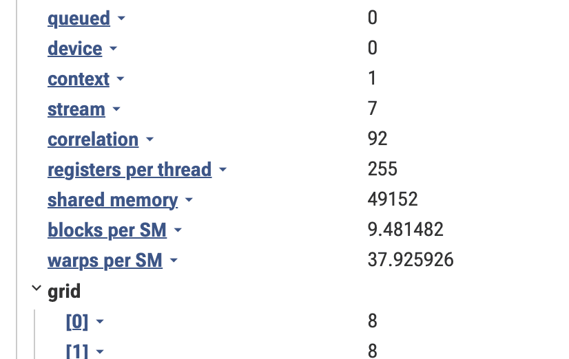
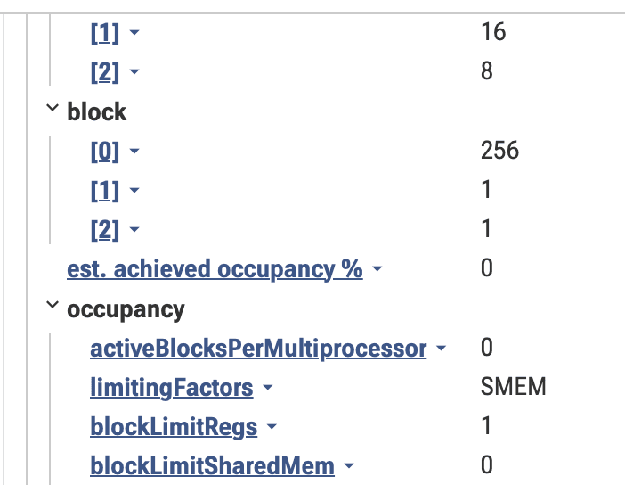
แม้ค่า occupancy จะดูต่ำ (รูปที่ 16-17) แต่นั่นเป็นเพราะ Flash Attention จงใจใช้ทรัพยากรบนชิป (Registers และ Shared Memory) อย่างหนักเพื่อเพิ่มประสิทธิภาพการประมวลผลให้สูงสุดโดยไม่ต้องพึ่งพา Global Memory
cuDNN backend
cuDNN จะสร้าง kernel ขึ้นมาแบบเฉพาะเจาะจงตามรูปร่างข้อมูล (codegen) ทำให้ชื่อ kernel มีรายละเอียดมาก (รูปที่ 18)
ความแตกต่างสำคัญคือ cuDNN สามารถจัดการข้อมูลโดยไม่ต้องทำ transpose (รูปที่ 19-21) และเรียกใช้ผ่าน driver-level API (cuLaunchKernelEx) อย่างไรก็ตาม ต้นทุนการคำนวณถูกย้ายไปที่ฝั่ง CPU แทนเพื่อเตรียมแผนการรัน (Knob search) ทำให้เสียเวลา CPU สูงกว่าแบบอื่น (รูปที่ 22-23)
บทสรุปของซีรีส์
บทเรียนสำคัญที่สุดคือ "เดาก่อน แล้วค่อยดู" การทำ Profiling ไม่ใช่เรื่องน่าเกรงขามสำหรับผู้เชี่ยวชาญเท่านั้น แต่คือระเบียบวินัยในการสังเกตความไม่สอดคล้องกันระหว่างผลลัพธ์ที่คาดหวังกับการทำงานจริงของฮาร์ดแวร์
| Variant | Kernels / forward | บทเรียนสำคัญ |
|---|---|---|
| Naive in-place | 5 | ลด Memcpy ได้ด้วยการเปลี่ยนโค้ดเพียงบรรทัดเดียว |
| SDPA math | 20 | ช้าแต่ชัวร์ ไม่ใช้ Tensor Cores และปลอดภัยสูงสุด |
| SDPA efficient | 1 | ใช้ fmha_cutlassF ยุบรวมการทำงานอย่างมีประสิทธิภาพ |
| SDPA flash | 1 | เร็วที่สุดในสภาพแวดล้อมที่เหมาะสม แม้ค่า occupancy จะดูต่ำ |
| SDPA cuDNN | 1 | ปรับแต่งมาเพื่อปัญหาเฉพาะหน้า แต่เสียเวลาฝั่ง CPU ในการวางแผน |
ตอนนี้คุณมีทักษะพร้อมที่จะวิเคราะห์โมเดลของคุณเองแล้ว! มาร่วมสนุกกับการทำ profiling กันเถอะ 🤗
ขอขอบคุณ Noe Flandre สำหรับการรีวิวเนื้อหา!









ความคิดเห็น (0)
เข้าสู่ระบบเพื่อร่วมแสดงความเห็น
สมัครสมาชิกมาเป็นคนแรกที่แสดงความเห็นกันเลยโบร