
จาก In-Silico สู่ Wet-Lab: เจาะลึกการใช้ AI ออกแบบโปรตีนและเกณฑ์วัดผลที่มีประสิทธิภาพ
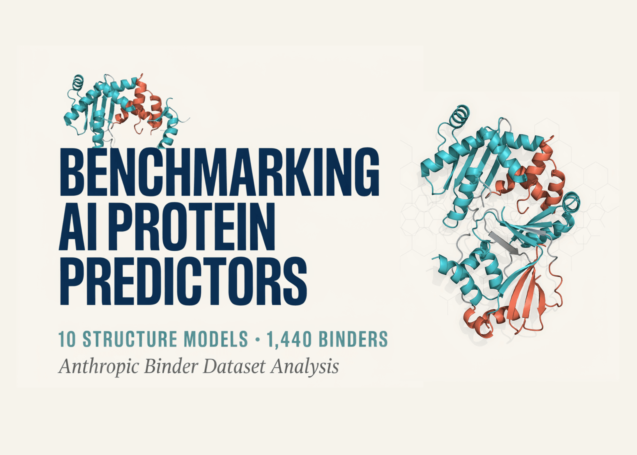
ในบทเรียนนี้ เราจะวิเคราะห์ชุดข้อมูล Anthropic’s claude-protein-binder-design ซึ่งประกอบด้วยโปรตีนขนาดเล็ก (miniprotein binder) ที่ออกแบบด้วย AI จำนวน 1,440 รายการ โดยผ่านการทดสอบกับเป้าหมาย (target) 16 ชนิด ข้อมูลนี้มีความพิเศษเนื่องจากรวมทั้งผลการทำนายเชิงคำนวณและผลลัพธ์จริงจากห้องปฏิบัติการอิสระ (wet-lab) สองแห่ง ทำให้เราสามารถประเมินได้ว่าเครื่องมือทำนายโครงสร้างระบุ binder ที่ประสบความสำเร็จได้แม่นยำเพียงใด รวมถึงผลกระทบจากการรวมการทำนาย (ensemble) และความคลาดเคลื่อนที่เกิดจากตัวแปรในการทดสอบ (assay)
import subprocess, sys, warnings, itertools, math
warnings.filterwarnings("ignore")
import importlib.util
_needed = {"huggingface_hub": "huggingface_hub>=0.24", "pyarrow": "pyarrow",
"pandas": "pandas", "sklearn": "scikit-learn",
"matplotlib": "matplotlib", "scipy": "scipy"}
_missing = [pkg for mod, pkg in _needed.items() if importlib.util.find_spec(mod) is None]
if _missing:
print("installing:", ", ".join(_missing))
subprocess.run([sys.executable, "-m", "pip", "install", "-q", *_missing], check=False)
import numpy as np
import pandas as pd
import matplotlib.pyplot as plt
from scipy import stats
from huggingface_hub import HfApi, hf_hub_download
from sklearn.metrics import roc_auc_score, cohen_kappa_score, average_precision_score
from sklearn.model_selection import GroupKFold, StratifiedKFold
from sklearn.ensemble import HistGradientBoostingClassifier
from sklearn.inspection import permutation_importance
SEED = 0
rng_global = np.random.default_rng(SEED)
pd.set_option("display.width", 200)
pd.set_option("display.max_columns", 100)
plt.rcParams.update({"figure.dpi": 110, "font.size": 9, "axes.grid": True,
"grid.alpha": 0.25, "axes.spines.top": False, "axes.spines.right": False})
REPO = "Anthropic/claude-protein-binder-design"
BAR = "=" * 78
def head(n, title):
prefix = f"{n}. " if str(n) else ""
print(f"\n{BAR}\n {prefix}{title}\n{BAR}")
head(1, "TABLE DISCOVERY")
api = HfApi()
repo_files = api.list_repo_files(REPO, repo_type="dataset")
TABLES = {}
for f in repo_files:
if f.startswith("data/tables/") and f.endswith(".parquet"):
key = f[len("data/tables/"): -len(".parquet")].replace("/", "_")
TABLES[key] = f
print(f"Found {len(TABLES)} Parquet tables:")
for k in sorted(TABLES):
print(f" - {k:38s} {TABLES[k]}")
def load_table(name: str) -> pd.DataFrame:
"""Load a subset by its viewer name, with a datasets-library fallback."""
if name in TABLES:
return pd.read_parquet(hf_hub_download(REPO, TABLES[name], repo_type="dataset"))
from datasets import load_dataset
return load_dataset(REPO, name, split="full").to_pandas()
ds = load_table("design_summary")
print(f"\ndesign_summary: {ds.shape[0]:,} rows x {ds.shape[1]} columns")
ขั้นตอนแรกเริ่มจากการเตรียมสภาพแวดล้อมและดึงข้อมูลจาก repository โดยเราใช้วิธีสร้างแผนผังไฟล์เพื่อป้องกันปัญหาการตั้งชื่อไฟล์ที่ไม่สม่ำเสมอ ข้อมูลหลักที่นำมาใช้คือ design_summary ซึ่งมีข้อมูลการออกแบบ 1,440 รายการ ครอบคลุมรายละเอียดที่จำเป็นสำหรับการวิเคราะห์ในขั้นตอนถัดไปทั้งหมด
head(2, "SCHEMA + EVALUABLE SET")
CALLS = {"binder", "non_binder"}
tested = ds["adaptyv_binding"].isin(CALLS) | ds["twist_binding"].isin(CALLS)
ev = ds[tested].copy()
ev["y"] = ev["binder_final"].astype(int)
print(f"All designs : {len(ds):,}")
print(f"Evaluable (>=1 vendor call): {len(ev):,}")
print(f"Confirmed binders : {int(ev['y'].sum()):,} "
f"({100 * ev['y'].mean():.1f}% base rate)")
print(f"Never measured : {len(ds) - len(ev):,}")
print("\nCategorical levels:")
for c in ["design_model", "campaign", "generator", "sequence_design_method", "vendor_agreement"]:
vals = ds[c].astype(str).value_counts()
print(f" {c:24s} ({len(vals)}): {', '.join(vals.index[:6])}"
+ (" ..." if len(vals) > 6 else ""))
print(f"\nTargets ({ds['target'].nunique()}): {', '.join(sorted(ds['target'].unique()))}")
print(f"Binder length: {ds.binder_length.min()}-{ds.binder_length.max()} aa "
f"(median {ds.binder_length.median():.0f})")
head(3, "HIT-RATE LANDSCAPE")
def wilson(k, n, z=1.96):
if n == 0:
return (np.nan, np.nan, np.nan)
p = k / n
d = 1 + z**2 / n
c = (p + z**2 / (2 * n)) / d
h = z * math.sqrt(p * (1 - p) / n + z**2 / (4 * n**2)) / d
return p, max(0.0, c - h), min(1.0, c + h)
def rate_table(df, by):
rows = []
for key, g in df.groupby(by, dropna=False):
p, lo, hi = wilson(int(g.y.sum()), len(g))
rows.append({by: key, "n": len(g), "hits": int(g.y.sum()),
"rate": p, "lo": lo, "hi": hi})
return pd.DataFrame(rows).sort_values("rate", ascending=False).reset_index(drop=True)
for dim in ["design_model", "campaign", "generator", "sequence_design_method"]:
t = rate_table(ev, dim)
print(f"\n--- hit rate by {dim} ---")
print(t.to_string(index=False,
formatters={"rate": "{:.3f}".format, "lo": "{:.3f}".format, "hi": "{:.3f}".format}))
tt = rate_table(ev, "target")
fig, ax = plt.subplots(figsize=(9, 4.2))
ax.bar(tt.target, tt.rate, color="#4C72B0")
ax.errorbar(tt.target, tt.rate,
yerr=[(tt.rate - tt.lo).clip(lower=0), (tt.hi - tt.rate).clip(lower=0)],
fmt="none", ecolor="0.25", capsize=3, lw=1)
ax.axhline(ev.y.mean(), ls="--", c="crimson", lw=1, label=f"pooled {ev.y.mean():.2f}")
ax.set_ylabel("experimental hit rate"); ax.set_title("Hit rate by target (Wilson 95% CI)")
ax.tick_params(axis="x", rotation=55); ax.legend(); plt.tight_layout(); plt.show()
print("\nRead this plot as the dominant effect size in the dataset: target choice "
"swamps generator choice. Any model comparison that does not stratify by "
"target is mostly measuring which targets that model was pointed at.")
การกำหนดเซตข้อมูลสำหรับการประเมิน (evaluable set) จะยึดตามผลลัพธ์จริงจาก vendor เพื่อความแม่นยำ จากนั้นจึงคำนวณอัตราการพบ (hit rates) โดยใช้ช่วง Wilson เพื่อลดความคลาดเคลื่อนในกลุ่มตัวอย่างน้อย ผลลัพธ์ยืนยันว่า "การเลือกแอนติเจนเป้าหมาย" ส่งผลต่อความสำเร็จมากกว่าปัจจัยอื่นๆ ทั้งหมด ซึ่งเป็นประเด็นสำคัญที่นักออกแบบโปรตีนต้องพึงระวัง
head(4, "PER-PREDICTOR DISCRIMINATIVE POWER")
PREDICTORS = sorted({c[len("ipsae_min_"):] for c in ds.columns if c.startswith("ipsae_min_")})
print(f"Predictors ({len(PREDICTORS)}): {', '.join(PREDICTORS)}")
def auc_ci(y, s, n_boot=300, seed=SEED):
s = np.asarray(s, dtype=float); y = np.asarray(y, dtype=int)
m = ~np.isnan(s)
y, s = y[m], s[m]
if len(y) < 30 or len(np.unique(y)) < 2:
return dict(auc=np.nan, lo=np.nan, hi=np.nan, n=len(y), ap=np.nan)
base = roc_auc_score(y, s)
ap = average_precision_score(y, s)
rng = np.random.default_rng(seed)
idx, boots = np.arange(len(y)), []
for _ in range(n_boot):
b = rng.choice(idx, len(idx), replace=True)
if len(np.unique(y[b])) > 1:
boots.append(roc_auc_score(y[b], s[b]))
lo, hi = (np.percentile(boots, [2.5, 97.5]) if boots else (np.nan, np.nan))
return dict(auc=base, lo=lo, hi=hi, n=len(y), ap=ap)
rows = []
for p in PREDICTORS:
for metric in ["ipsae_min", "sc_dockq"]:
col = f"{metric}_{p}"
if col in ev.columns:
r = auc_ci(ev.y, ev[col])
rows.append({"predictor": p, "metric": metric, **r})
perf = pd.DataFrame(rows)
piv = perf.pivot(index="predictor", columns="metric", values="auc").sort_values("ipsae_min", ascending=False)
print("\nAUC vs experimental binder_final:")
print(perf.sort_values("auc", ascending=False).to_string(
index=False, formatters={c: "{:.3f}".format for c in ["auc", "lo", "hi", "ap"]}))
fig, ax = plt.subplots(figsize=(9, 4.2))
x = np.arange(len(piv)); w = 0.38
for i, (metric, colr) in enumerate([("ipsae_min", "#4C72B0"), ("sc_dockq", "#DD8452")]):
sub = perf[perf.metric == metric].set_index("predictor").reindex(piv.index)
lo_err = (sub.auc - sub.lo).clip(lower=0).fillna(0)
hi_err = (sub.hi - sub.auc).clip(lower=0).fillna(0)
ax.bar(x + (i - 0.5) * w, sub.auc, w, label=metric, color=colr)
ax.errorbar(x + (i - 0.5) * w, sub.auc,
yerr=[lo_err, hi_err], fmt="none", ecolor="0.3", capsize=2, lw=0.9)
ax.axhline(0.5, ls="--", c="crimson", lw=1)
ax.set_xticks(x); ax.set_xticklabels(piv.index, rotation=45, ha="right")
ax.set_ylabel("AUC"); ax.set_ylim(0.35, None)
ax.set_title("In-silico score vs wet-lab binding, by structure predictor")
ax.legend(); plt.tight_layout(); plt.show()
print("Interpretation: AUCs land well above chance but far below the ~0.9 you "
"would need to trust a single filter. That gap is the entire practical "
"reason this dataset exists.")
head(5, "CONSENSUS SCORING")
ips_cols = [f"ipsae_min_{p}" for p in PREDICTORS if f"ipsae_min_{p}" in ev.columns]
dq_cols = [f"sc_dockq_{p}" for p in PREDICTORS if f"sc_dockq_{p}" in ev.columns]
def pct_rank(df, cols):
return df[cols].rank(pct=True, na_option="keep")
R_ips, R_dq = pct_rank(ev, ips_cols), pct_rank(ev, dq_cols)
ev["cons_ipsae"] = R_ips.mean(axis=1)
ev["cons_dockq"] = R_dq.mean(axis=1)
ev["cons_all"] = pd.concat([R_ips, R_dq], axis=1).mean(axis=1)
ev["cons_median"] = pd.concat([R_ips, R_dq], axis=1).median(axis=1)
ev["cons_min"] = pd.concat([R_ips, R_dq], axis=1).min(axis=1)
ev["cons_disagree"] = pd.concat([R_ips, R_dq], axis=1).std(axis=1)
best_single = perf.loc[perf.auc.idxmax()]
print(f"Best single column: {best_single.metric}_{best_single.predictor} AUC={best_single.auc:.3f}")
print()
for name in ["cons_ipsae", "cons_dockq", "cons_all", "cons_median", "cons_min", "cons_disagree"]:
r = auc_ci(ev.y, ev[name])
print(f" {name:16s} AUC={r['auc']:.3f} [{r['lo']:.3f}, {r['hi']:.3f}] AP={r['ap']:.3f}")
corr = ev[ips_cols].corr(method="spearman")
fig, ax = plt.subplots(figsize=(6.2, 5.2))
im = ax.imshow(corr.values, cmap="viridis", vmin=0, vmax=1)
lbl = [c.replace("ipsae_min_", "") for c in ips_cols]
ax.set_xticks(range(len(lbl))); ax.set_xticklabels(lbl, rotation=90)
ax.set_yticks(range(len(lbl))); ax.set_yticklabels(lbl)
ax.set_title("Spearman correlation between predictors (ipSAE)")
ax.grid(False); fig.colorbar(im, shrink=0.8); plt.tight_layout(); plt.show()
print("\nIf every off-diagonal cell were ~1.0 there would be no ensemble gain to "
"harvest. The moderate correlations are why cons_all typically edges out "
"the best single predictor — and why disagreement itself carries signal.")
เราประเมินประสิทธิภาพของตัวทำนายทั้ง 10 รายการ โดยใช้เมตริก ipSAE และความสอดคล้องของโครงสร้าง (self-consistency) ผลลัพธ์ค่า AUC ชี้ให้เห็นว่าแม้ผลการทำนายจะดีกว่าการสุ่ม แต่ก็ยังไม่แม่นยำพอที่จะใช้เป็นตัวกรองหลักเพียงอย่างเดียว อย่างไรก็ตาม การใช้วิธี Consensus Scoring หรือการเฉลี่ยอันดับจากหลายโมเดล ช่วยเพิ่มประสิทธิภาพในการจำแนก binder ได้ดีขึ้น เนื่องจากตัวทำนายแต่ละตัวมีความเหลื่อมล้ำในการวิเคราะห์ (moderate correlation)
head(6, "BUDGET CURVES (precision@N)")
def budget_curve(df, score_col, max_n=400):
d = df[[score_col, "y"]].dropna().sort_values(score_col, ascending=False)
hits = d.y.values.cumsum()
n = np.arange(1, len(d) + 1)
k = min(max_n, len(d))
return n[:k], (hits / n)[:k]
fig, ax = plt.subplots(figsize=(8, 4.4))
best_col = f"{best_single.metric}_{best_single.predictor}"
for col, lab, style in [(best_col, f"best single ({best_col})", "-"),
("cons_all", "consensus (rank-avg, all)", "-"),
("cons_min", "consensus (unanimity/min)", "--")]:
n, prec = budget_curve(ev, col)
ax.plot(n, prec, style, lw=1.8, label=lab)
ax.axhline(ev.y.mean(), ls=":", c="crimson", lw=1.4, label=f"random baseline ({ev.y.mean():.2f})")
ax.set_xlabel("designs ordered for wet-lab testing (N, best-first)")
ax.set_ylabel("hit rate among top N"); ax.set_title("How much does in-silico triage buy you?")
ax.legend(); plt.tight_layout(); plt.show()
print("Enrichment at small budgets:")
for N in [25, 50, 100, 200]:
line = f" N={N:4d} | random {ev.y.mean():.3f}"
for col, lab in [(best_col, "best-single"), ("cons_all", "consensus")]:
n, prec = budget_curve(ev, col, max_n=N)
line += f" | {lab} {prec[-1]:.3f} ({prec[-1] / ev.y.mean():.2f}x)"
print(line)
head(7, "VENDOR CONCORDANCE")
both = ev[ev.adaptyv_binding.isin(CALLS) & ev.twist_binding.isin(CALLS)]
ct = pd.crosstab(both.adaptyv_binding, both.twist_binding)
print(f"Designs with calls from BOTH vendors: {len(both):,}\n")
print(ct.to_string())
if len(both) > 10:
kappa = cohen_kappa_score(both.adaptyv_binding, both.twist_binding)
agree = (both.adaptyv_binding == both.twist_binding).mean()
print(f"\nRaw agreement: {agree:.3f} Cohen's kappa: {kappa:.3f}")
print("Kappa well under 1.0 means part of the 'unpredictable' variance above "
"is assay disagreement, not model failure.")
kd = ev[["adaptyv_kd_nM", "twist_kd_nM"]].dropna()
kd = kd[(kd > 0).all(axis=1)]
if len(kd) > 10:
rho, pv = stats.spearmanr(kd.adaptyv_kd_nM, kd.twist_kd_nM)
fig, ax = plt.subplots(figsize=(4.8, 4.6))
ax.scatter(kd.adaptyv_kd_nM, kd.twist_kd_nM, s=16, alpha=0.6, c="#4C72B0", edgecolor="none")
lims = [min(kd.min()) * 0.5, max(kd.max()) * 2]
ax.plot(lims, lims, "k--", lw=1)
ax.set_xscale("log"); ax.set_yscale("log")
ax.set_xlabel("Adaptyv KD (nM)"); ax.set_ylabel("Twist KD (nM)")
ax.set_title(f"Cross-vendor KD, n={len(kd)}, Spearman rho={rho:.2f}")
plt.tight_layout(); plt.show()
med_ratio = np.median(kd.twist_kd_nM / kd.adaptyv_kd_nM)
print(f"Median KD ratio (Twist/Adaptyv): {med_ratio:.2f}x -> systematic format offset, "
"so treat absolute KD across vendors as ordinal, not interchangeable.")
เมื่อวิเคราะห์ในเชิงเศรษฐศาสตร์ผ่านกราฟ Precision@N เราพบว่าการคัดกรองเบื้องต้น (triage) ช่วยเพิ่มประสิทธิภาพได้อย่างมากเมื่อเทียบกับงบประมาณที่จำกัด นอกจากนี้ การเปรียบเทียบผลระหว่างสองห้องปฏิบัติการ (Adaptyv และ Twist) แสดงให้เห็นว่ามีความไม่สอดคล้องกันของข้อมูลการทดสอบ (assay disagreement) อยู่บ้าง ซึ่งถือเป็นเพดานสำคัญที่จำกัดความแม่นยำในการทำนายของโมเดล
head(8, "EXPRESSION CONFOUND")
if "twist_expression_mg_per_mL" in ev.columns:
g = ev.dropna(subset=["twist_expression_mg_per_mL"])
a = g.loc[g.y == 1, "twist_expression_mg_per_mL"]
b = g.loc[g.y == 0, "twist_expression_mg_per_mL"]
if len(a) > 5 and len(b) > 5:
u, pv = stats.mannwhitneyu(a, b)
print(f"Titer (mg/mL) binders median {a.median():.2f} (n={len(a)}) | "
f"non-binders {b.median():.2f} (n={len(b)}) Mann-Whitney p={pv:.2e}")
r = auc_ci(g.y, g.twist_expression_mg_per_mL)
print(f"AUC of raw expression titer alone as a 'binder' predictor: {r['auc']:.3f}")
fig, axes = plt.subplots(1, 2, figsize=(9, 3.6))
axes[0].hist([b, a], bins=25, label=["non-binder", "binder"],
color=["#BBBBBB", "#4C72B0"], density=True)
axes[0].set_xlabel("Twist titer (mg/mL)"); axes[0].set_ylabel("density"); axes[0].legend()
axes[0].set_title("Expression by outcome")
if "adaptyv_expression" in ev.columns:
ex = ev.groupby(ev.adaptyv_expression.astype(str)).y.agg(["mean", "size"])
ex = ex[ex["size"] >= 10].sort_values("mean")
axes[1].barh(ex.index, ex["mean"], color="#DD8452")
axes[1].set_xlabel("hit rate"); axes[1].set_title("Hit rate by Adaptyv expression class")
plt.tight_layout(); plt.show()
print("\nTakeaway: if expression alone scores meaningfully above 0.5, then part of "
"every AUC in section 4 is a solubility signal riding along. To isolate "
"interface quality, re-run section 4 restricted to designs that expressed.")
expressed = ev[ev.adaptyv_expression.astype(str).isin(["medium", "high"])] if "adaptyv_expression" in ev.columns else ev
if len(expressed) > 100:
r_all = auc_ci(ev.y, ev.cons_all)
r_exp = auc_ci(expressed.y, expressed.cons_all)
print(f" consensus AUC, all evaluable : {r_all['auc']:.3f} (n={r_all['n']})")
print(f" consensus AUC, expressed only : {r_exp['auc']:.3f} (n={r_exp['n']})")
head(9, "EPITOPE CONVERGENCE")
def parse_epitope(s):
if not isinstance(s, str) or not s.strip():
return frozenset()
out = set()
for tok in s.split(";"):
tok = tok.strip()
if not tok:
continue
out.add(tok.split(":")[-1])
return frozenset(out)
ev["epi"] = ev["epitope_residues"].apply(parse_epitope)
def mean_pairwise_jaccard(sets, max_pairs=4000, seed=SEED):
sets = [s for s in sets if len(s) > 0]
if len(sets) < 2:
return np.nan
pairs = list(itertools.combinations(range(len(sets)), 2))
rng = np.random.default_rng(seed)
if len(pairs) > max_pairs:
pairs = [pairs[i] for i in rng.choice(len(pairs), max_pairs, replace=False)]
vals = []
for i, j in pairs:
u = len(sets[i] | sets[j])
vals.append(len(sets[i] & sets[j]) / u if u else 0.0)
return float(np.mean(vals))
row = []
for tgt, g in ev.groupby("target"):
B = g.loc[g.y == 1, "epi"].tolist()
N = g.loc[g.y == 0, "epi"].tolist()
if len(B) >= 3 and len(N) >= 3:
rows.append({"target": tgt, "n_bind": len(B), "n_non": len(N),
"J_binders": mean_pairwise_jaccard(B),
"J_nonbinders": mean_pairwise_jaccard(N)})
epi = pd.DataFrame(rows)
if len(epi):
epi["delta"] = epi.J_binders - epi.J_nonbinders
print(epi.sort_values("delta", ascending=False).to_string(
index=False, formatters={c: "{:.3f}".format for c in ["J_binders", "J_nonbinders", "delta"]}))
w = stats.wilcoxon(epi.J_binders, epi.J_nonbinders) if len(epi) >= 6 else None
if w:
print(f"\nPaired Wilcoxon across targets: p={w.pvalue:.4f} "
f"(binders more epitope-convergent than failures?)")
tgt = epi.sort_values("n_bind", ascending=False).target.iloc[0]
sub = ev[ev.target == tgt]
freq_b = pd.Series([r for s in sub[sub.y == 1].epi for r in s]).value_counts()
freq_n = pd.Series([r for s in sub[sub.y == 0].epi for r in s]).value_counts()
top = freq_b.head(18).index
fig, ax = plt.subplots(figsize=(9, 3.8))
xx = np.arange(len(top))
ax.bar(xx - 0.2, (freq_b.reindex(top).fillna(0) / max(1, (sub.y == 1).sum())), 0.4,
label="binders", color="#4C72B0")
ax.bar(xx + 0.2, (freq_n.reindex(top).fillna(0) / max(1, (sub.y == 0).sum())), 0.4,
label="non-binders", color="#BBBBBB")
ax.set_xticks(xx); ax.set_xticklabels(top, rotation=70, ha="right")
ax.set_ylabel("fraction of designs contacting"); ax.set_title(f"Epitope usage on {tgt}")
ax.legend(); plt.tight_layout(); plt.show()
การวิเคราะห์ยังเผยให้เห็นว่า ปริมาณการแสดงออก (expression titer) มีความสัมพันธ์กับความสำเร็จในการจับตัว (binding) ซึ่งหมายความว่าความล้มเหลวบางส่วนอาจไม่ได้เกิดจากโครงสร้างการจับไม่ดี แต่เกิดจากการที่โปรตีนไม่ละลายหรือแสดงออกน้อยเกินไป นอกจากนี้ยังพบว่า binder ที่ประสบความสำเร็จมักจะมีจุดสัมผัส (epitope) ในบริเวณเดียวกันมากกว่ากลุ่มที่ล้มเหลว
head(10, "MODELLING WITH HONEST CROSS-VALIDATION")
AAS = "ACDEFGHIKLMNPQRSTVWY"
KD_HYDRO = dict(zip(AAS, [1.8, 2.5, -3.5, -3.5, 2.8, -0.4, -3.2, 4.5, -3.9, 3.8,
1.9, -3.5, -1.6, -3.5, -4.5, -0.8, -0.7, 4.2, -0.9, -1.3]))
CHARGE = {"K": 1, "R": 1, "H": 0.1, "D": -1, "E": -1}
def seq_features(seq):
seq = "".join(ch for ch in str(seq).upper() if ch in AAS)
L = max(1, len(seq))
counts = {a: seq.count(a) / L for a in AAS}
f = {f"aa_{a}": counts[a] for a in AAS}
f["length"] = len(seq)
f["net_charge"] = sum(CHARGE.get(c, 0) for c in seq)
f["charge_density"] = f["net_charge"] / L
f["gravy"] = float(np.mean([KD_HYDRO[c] for c in seq])) if seq else 0.0
f["aromatic"] = sum(counts[a] for a in "FWY")
f["helix_prone"] = sum(counts[a] for a in "AELM")
f["beta_prone"] = sum(counts[a] for a in "VIYFT")
f["gly_pro"] = counts["G"] + counts["P"]
p = np.array([counts[a] for a in AAS]); p = p[p > 0]
f["entropy"] = float(-(p * np.log2(p)).sum())
run, best = 0, 0
for c in seq:
run = run + 1 if KD_HYDRO[c] > 1.5 else 0
best = max(best, run)
f["max_hydrophobic_run"] = best
return f
SF = pd.DataFrame([seq_features(s) for s in ev.sequence], index=ev.index)
seq_cols = list(SF.columns)
sil_cols = [c for c in ev.columns if c.startswith(("ipsae_min_", "sc_dockq_"))] + \
["cons_all", "cons_min", "cons_disagree"]
meta_cols = [c for c in ["rank", "n_optimization_rounds", "epitope_n_residues"] if c in ev.columns]
X_all = pd.concat([ev[sil_cols + meta_cols], SF], axis=1)
y = ev.y.values
groups = ev.target.values
FEATURE_SETS = {
"in-silico only": sil_cols + meta_cols,
"sequence only": seq_cols,
"in-silico + sequence": sil_cols + meta_cols + seq_cols,
}
def cv_auc(X, y, splitter, groups=None):
aucs = []
it = splitter.split(X, y, groups) if groups is not None else splitter.split(X, y)
for tr, te in it:
if len(np.unique(y[te])) < 2:
continue
m = HistGradientBoostingClassifier(max_depth=4, max_iter=250,
learning_rate=0.06, random_state=SEED)
m.fit(X.iloc[tr], y[tr])
aucs.append(roc_auc_score(y[te], m.predict_proba(X.iloc[te])[:, 1]))
return float(np.mean(aucs)), float(np.std(aucs)), len(aucs)
print(f"{'feature set':24s} {'random 5-fold':>18s} {'grouped-by-target':>20s}")
print("-" * 66)
results = {}
for name, cols in FEATURE_SETS.items():
X = X_all[cols]
r_mean, r_sd, _ = cv_auc(X, y, StratifiedKFold(5, shuffle=True, random_state=SEED))
g_mean, g_sd, nf = cv_auc(X, y, GroupKFold(n_splits=5), groups=groups)
results[name] = (r_mean, g_mean)
print(f"{name:24s} {r_mean:.3f} +/- {r_sd:.3f} {g_mean:.3f} +/- {g_sd:.3f}")
gap = results["in-silico + sequence"][0] - results["in-silico + sequence"][1]
print(f"\nRandom-CV minus grouped-CV for the full feature set: {gap:+.3f}")
print("That gap is leakage: features that encode target identity (epitope size, "
"length priors, generator habits) let a randomly-split model recover the "
"per-target base rate instead of learning what makes a binder. Report the "
"grouped number; the random one is what a target-blind reviewer will catch.")
Xt = pd.get_dummies(pd.Series(groups, index=ev.index), prefix="tgt")
r_mean, _, _ = cv_auc(Xt, y, StratifiedKFold(5, shuffle=True, random_state=SEED))
print(f"\nControl - target one-hot ONLY, random CV: AUC={r_mean:.3f} "
"(pure base-rate memorisation, zero design signal).")
gkf = GroupKFold(n_splits=5)
tr, te = next(iter(gkf.split(X_all, y, groups)))
model = HistGradientBoostingClassifier(max_depth=4, max_iter=250,
learning_rate=0.06, random_state=SEED).fit(
X_all[FEATURE_SETS["in-silico + sequence"]].iloc[tr], y[tr])
imp = permutation_importance(model, X_all[FEATURE_SETS["in-silico + sequence"]].iloc[te],
y[te], n_repeats=12, random_state=SEED, scoring="roc_auc")
order = np.argsort(imp.importances_mean)[-18:]
names = np.array(FEATURE_SETS["in-silico + sequence"])[order]
fig, ax = plt.subplots(figsize=(7, 5))
ax.barh(names, imp.importances_mean[order],
xerr=imp.importances_std[order], color="#55A868")
ax.set_xlabel("drop in AUC when permuted")
ax.set_title("Permutation importance (held-out target block)")
plt.tight_layout(); plt.show()
head("", "SUMMARY")
print(f"""
Evaluable designs : {len(ev):,} base hit rate {ev.y.mean():.3f}
Best single in-silico : {best_col} AUC {best_single.auc:.3f}
Rank-average consensus : AUC {auc_ci(ev.y, ev.cons_all)['auc']:.3f}
Honest ML (grouped CV) : AUC {results['in-silico + sequence'][1]:.3f} <- the one to report
Same model, random CV : AUC {results['in-silico + sequence'][0]:.3f} (gap = {gap:+.3f} leakage)
Five things this dataset teaches that a design paper usually cannot:
1. Target identity dominates every other factor; always stratify.
2. Structure-predictor confidence is real but weak signal (AUC ~0.6-0.75),
nowhere near a standalone go/no-go filter.
3. Ensembling across predictors is a cheap, reliable few-points-of-AUC win.
4. Cross-vendor label noise caps how high any AUC here can honestly go.
5. Expression failure masquerades as binding failure. Condition on it.
Extensions worth trying:
- load_table('insilico_cofold_predictions') for all 5 seeds/predictor, and
test whether seed VARIANCE beats seed-best as a confidence signal
- load_table('adaptyv_fit_curves') to refit kinetics yourself and flag
designs whose reported KD rests on a poorly-conditioned fit
- load_table('insilico_provenance_steps') to relate optimisation-round count
to eventual success
- snapshot_download(..., allow_patterns='data/designs/EGFR/<name>/*') for
mmCIF structures + PAE matrices on a single design
""")
บทสรุปจากการวิเคราะห์ย้ำว่า การประเมินประสิทธิภาพการออกแบบโปรตีนด้วย AI ต้องทำอย่างรัดกุม โดยเฉพาะการทำ Cross-Validation ที่ต้องแบ่งกลุ่มตามเป้าหมาย (target-grouped folds) เพื่อป้องกันปัญหาข้อมูลรั่วไหล (leakage) และให้ผลลัพธ์ที่นำไปใช้งานได้จริงกับเป้าหมายใหม่ๆ ในอนาคต
การศึกษาครั้งนี้สอนให้เรารู้ว่า: 1) เป้าหมายมีความสำคัญสูงสุด 2) ความแม่นยำของตัวทำนายโครงสร้างยังอยู่ในระดับกลาง 3) การทำ ensemble ช่วยเพิ่มประสิทธิภาพได้ 4) สัญญาณรบกวนจากการทดลองมีผลต่อค่าความแม่นยำ และ 5) ต้องแยกแยะปัญหาการแสดงออกออกจากความล้มเหลวในการจับตัวให้ได้
ความคิดเห็น (0)
เข้าสู่ระบบเพื่อร่วมแสดงความเห็น
สมัครสมาชิกมาเป็นคนแรกที่แสดงความเห็นกันเลยโบร