
สร้างระบบพยากรณ์อากาศ Ensemble แบบ Batched ด้วย NVIDIA Earth2Studio
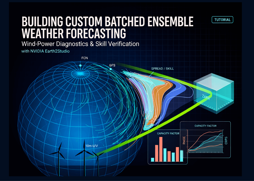
ใน บทช่วยสอน นี้ เราจะสร้างเวิร์กโฟลว์การพยากรณ์อากาศแบบ ensemble ด้วย NVIDIA Earth2Studio โดยเริ่มจากการติดตั้งส่วนประกอบที่จำเป็นในขณะที่ยังคงรักษาสภาพแวดล้อม PyTorch ที่รองรับ CUDA เดิมของ Colab ไว้ จากนั้นจึงโหลดโมเดลพยากรณ์ FCN และดึงข้อมูลสภาวะเริ่มต้นของชั้นบรรยากาศจาก GFS
ขั้นตอนถัดมาคือการปรับใช้การวินิจฉัยพลังงานลมแบบกำหนดเอง ที่แปลงองค์ประกอบลมระดับ 10 เมตรให้เป็นปัจจัยความสามารถในการผลิตของกังหัน (capacity factors) พร้อมระบบรบกวนข้อมูล (perturbation system) แบบปรับขนาดตัวแปร ซึ่งใช้แอมพลิจูดสัญญาณรบกวนที่เหมาะสมทางกายภาพกับตัวแปรบรรยากาศต่างๆ โดยยังคงสมาชิกควบคุม (control member) ที่ไม่มีการรบกวนไว้
การสร้าง pipeline ครั้งนี้ใช้ low-level iterator, coordinate-mapping, batching และ Zarr APIs ของ Earth2Studio เพื่อเขียนฟิลด์การพยากรณ์และการวินิจฉัยลงในที่จัดเก็บข้อมูลที่รับรู้พิกัด (coordinate-aware data store) พร้อมตรวจสอบการพยากรณ์กับข้อมูลวิเคราะห์ GFS โดยใช้ RMSE แบบถ่วงน้ำหนักตามละติจูด, fair CRPS, ensemble spread และ spread-skill ratios ก่อนจะแสดงผลความไม่แน่นอนผ่านแผนที่เชิงพื้นที่, spaghetti plots, fan charts และกราฟทักษะตามระยะเวลาพยากรณ์ (lead-time skill curves)
import importlib.util, os, subprocess, sys
if importlib.util.find_spec("earth2studio") is None:
import numpy as _np, torch as _torch
cfile = os.path.join(os.getcwd(), "e2s_constraints.txt")
with open(cfile, "w") as f:
f.write(f"torch=={_torch.__version__.split('+')[0]}\n")
f.write(f"numpy=={_np.__version__}\n")
env = {**os.environ, "PIP_CONSTRAINT": cfile}
subprocess.check_call(
[sys.executable, "-m", "pip", "install", "-q",
"earth2studio[fcn,data,perturbation,statistics]"], env=env)
print("\n>>> Install done. If the imports below fail: Runtime > Restart session, re-run.\n")
os.environ.setdefault("EARTH2STUDIO_CACHE", "/content/e2s_cache")
os.makedirs("outputs", exist_ok=True)
from collections import OrderedDict
from datetime import datetime, timedelta, timezone
from tqdm.auto import tqdm
from earth2studio.data import GFS, fetch_data
from earth2studio.io import ZarrBackend
from earth2studio.models.batch import batch_coords, batch_func
from earth2studio.models.px import FCN
from earth2studio.statistics import rmse
from earth2studio.utils import handshake_coords, handshake_dim
from earth2studio.utils.coords import map_coords
from earth2studio.utils.time import to_time_array
from earth2studio.utils.type import CoordSystem
if DEVICE.type == "cpu":
print("!! No GPU detected — this will be very slow. Runtime > Change runtime type > T4 GPU")
NENSEMBLE = 8
BATCH_SIZE = 2
NSTEPS = 8
SAVE_VARS = ["t2m", "z500", "u10m", "v10m", "tcwv"]
VERIFY_VARS = ["t2m", "z500", "u10m"]
INIT = (datetime.now(timezone.utc) - timedelta(days=7)).replace()
INIT_STR = INIT.strftime("%Y-%m-%dT%H:%M:%S")
POI = ("New Delhi", 28.61, 77.21)
print(f"Initialization: {INIT_STR} | device: {DEVICE}")
เราเริ่มจากการติดตั้ง Earth2Studio โดยใช้ package constraints เพื่อรักษาเวอร์ชันของ PyTorch และ NumPy ที่รองรับ CUDA ของ Colab ไว้ จากนั้นจึงกำหนดค่า cache ของโมเดล นำเข้ายูทิลิตี้การพยากรณ์ ข้อมูล สถิติ และการจัดการพิกัด พร้อมระบุพารามิเตอร์สำคัญ เช่น ขนาด ensemble, ขนาด batch, ระยะเวลาพยากรณ์ และจุดที่สนใจในนิวเดลี
class WindPowerCF(torch.nn.Module):
"""Turbine capacity factor [0,1] from 10 m winds via power-law shear + power curve."""
def __init__(self, lat, lon, hub=100.0, alpha=0.143,
cut_in=3.0, rated=12.0, cut_out=25.0):
super().__init__()
self.lat, self.lon = lat, lon
self.hub, self.alpha = hub, alpha
self.cut_in, self.rated, self.cut_out = cut_in, rated, cut_out
def input_coords(self) -> CoordSystem:
return OrderedDict({
"batch": np.empty(0),
"variable": np.array(["u10m", "v10m"]),
"lat": self.lat,
"lon": self.lon,
})
@batch_coords()
def output_coords(self, input_coords: CoordSystem) -> CoordSystem:
target = self.input_coords()
for i, (key, _) in enumerate(target.items()):
if key != "batch":
handshake_dim(input_coords, key, i)
handshake_coords(input_coords, target, key)
oc = OrderedDict({
"batch": np.empty(0),
"variable": np.array(["wind_cf"]),
"lat": self.lat,
"lon": self.lon,
})
oc["batch"] = input_coords["batch"]
return oc
@batch_func()
def __call__(self, x: torch.Tensor, coords: CoordSystem):
oc = self.output_coords(coords)
u, v = x[..., 0:1, :, :], x[..., 1:2, :, :]
ws10 = torch.sqrt(u * u + v * v)
ws = ws10 * (self.hub / 10.0) ** self.alpha
ramp = (ws ** 3 - self.cut_in ** 3) / (self.rated ** 3 - self.cut_in ** 3)
cf = torch.zeros_like(ws)
cf = torch.where((ws >= self.cut_in) & (ws < self.rated), ramp.clamp(0, 1), cf)
cf = torch.where((ws >= self.rated) & (ws <= self.cut_out), torch.ones_like(cf), cf)
return cf, oc
class VariableScaledNoise:
"""Spatially correlated noise with per-variable amplitudes + control member."""
def __init__(self, amplitudes: dict, default: float = 0.0, control_member: bool = True):
self.amplitudes, self.default, self.control = amplitudes, default, control_member
try:
from earth2studio.perturbation import SphericalGaussian
self.sampler, self.kind = SphericalGaussian(noise_amplitude=1.0), "SphericalGaussian"
except Exception:
from earth2studio.perturbation import Brown
self.sampler, self.kind = Brown(noise_amplitude=1.0), "Brown"
def __call__(self, x: torch.Tensor, coords: CoordSystem):
noise, _ = self.sampler(torch.zeros_like(x), coords)
vax = list(coords).index("variable")
amps = torch.tensor([self.amplitudes.get(str(v), self.default)
for v in coords["variable"]], device=x.device, dtype=x.dtype)
shape = [1] * x.ndim; shape[vax] = amps.numel()
pert = noise * amps.reshape(shape)
if self.control and "ensemble" in coords:
eax = list(coords).index("ensemble")
mask = torch.tensor((np.asarray(coords["ensemble"]) != 0).astype(np.float32),
device=x.device, dtype=x.dtype)
mshape = [1] * x.ndim; mshape[eax] = mask.numel()
pert = pert * mask.reshape(mshape)
return x + pert, coords
เราสร้างโมเดลวินิจฉัยแบบกำหนดเองเพื่อแปลงองค์ประกอบลมระดับ 10 เมตร ให้เป็นความเร็วลมที่ความสูงดุมล้อและคำนวณปัจจัยการผลิตพลังงานของกังหัน โดยมีการตรวจสอบพิกัดผ่านระบบ handshake ของ Earth2Studio และรองรับการประมวลผลแบบ batch นอกจากนี้ยังนำการรบกวนเชิงพื้นที่มาใช้โดยรักษาค่าสมาชิกศูนย์ไว้เป็นตัวควบคุมหลัก
def write_vars(io, x, coords, names):
"""Write selected channels of a (…, variable, lat, lon) tensor to the IO backend."""
vax = list(coords).index("variable")
sub = OrderedDict((k, v) for k, v in coords.items() if k != "variable")
for name in names:
hit = np.where(np.asarray(coords["variable"]) == name)[0]
if hit.size:
io.write(x.select(vax, int(hit[0])).cpu(), sub, name)
def run_ensemble(time, nsteps, nensemble, batch_size, prognostic, diagnostic,
perturbation, data, io, save_vars, device):
time = to_time_array(time)
ic = prognostic.input_coords()
x0, c0 = fetch_data(source=data, time=time, lead_time=ic["lead_time"],
variable=ic["variable"], device=device)
print(f"Initial condition tensor: {tuple(x0.shape)} dims={list(c0)}")
oc = prognostic.output_coords(ic)
dt = oc["lead_time"]
prog_vars = [v for v in save_vars if v in set(map(str, oc["variable"]))]
total = OrderedDict({
"ensemble": np.arange(nensemble),
"time": time,
"lead_time": np.asarray([dt * i for i in range(nsteps + 1)]).flatten(),
"lat": oc["lat"],
"lon": oc["lon"],
})
io.add_array(total, prog_vars + ["wind_cf"])
dx_target = OrderedDict((k, v) for k, v in diagnostic.input_coords().items() if k != "batch")
nbatch = int(np.ceil(nensemble / batch_size))
with torch.inference_mode():
for b in tqdm(range(nbatch), desc="ensemble batches"):
lo = b * batch_size
n = min(batch_size, nensemble - lo)
x = x0.unsqueeze(0).repeat(n, *([1] * x0.ndim))
coords = OrderedDict({"ensemble": np.arange(lo, lo + n), **c0})
x, coords = perturbation(x, coords)
x, coords = map_coords(x, coords, ic)
for step, (xs, cs) in enumerate(prognostic.create_iterator(x, coords)):
write_vars(io, xs, cs, prog_vars)
xw, cw = map_coords(xs, cs, dx_target)
xw, cw = diagnostic(xw, cw)
write_vars(io, xw, cw, ["wind_cf"])
if step >= nsteps:
break
torch.cuda.empty_cache() if device.type == "cuda" else None
return io
model = FCN.load_model(FCN.load_default_package()).to(DEVICE)
grid = model.output_coords(model.input_coords())
LAT, LON = grid["lat"], grid["lon"]
diagnostic = WindPowerCF(LAT, LON).to(DEVICE)
pert = VariableScaledNoise(
amplitudes={"t2m": 0.20, "t850": 0.20, "z500": 40.0, "z850": 25.0,
"u10m": 0.25, "v10m": 0.25, "u500": 0.40, "v500": 0.40, "tcwv": 0.30},
default=0.0, control_member=True)
print(f"Perturbation sampler: {pert.kind}")
io = ZarrBackend(file_name="outputs/e2s_ensemble.zarr",
chunks={"ensemble": 1, "time": 1, "lead_time": 1},
backend_kwargs={"overwrite": True})
io = run_ensemble([INIT_STR], NSTEPS, NENSEMBLE, BATCH_SIZE,
model, diagnostic, pert, GFS(), io, SAVE_VARS, DEVICE)
print(io.root.tree())
เราสร้างฟังก์ชันช่วยเหลือเพื่อบันทึกข้อมูลบรรยากาศลงใน backend แบบ Zarr และออกแบบ loop สำหรับ ensemble แบบ batched ที่สามารถดึงสภาวะเริ่มต้น รบกวนสมาชิก จัดแนวพิกัด และเชื่อมต่อการวินิจฉัยพลังงานลมเข้ากับโมเดล FCN ได้อย่างต่อเนื่อง ก่อนจะดำเนินการพยากรณ์จริงและตรวจสอบโครงสร้างไฟล์ข้อมูลที่ได้
leads = np.asarray(io["lead_time"][:]).astype("timedelta64[ns]")
lead_h = leads.astype("timedelta64[h]").astype(int)
valid = to_time_array([INIT_STR])[0] + leads
truth, tc = fetch_data(source=GFS(), time=valid,
lead_time=np.array([np.timedelta64(0, "h")]),
variable=np.array(VERIFY_VARS), device="cpu")
truth = truth[:, 0]
w = torch.cos(torch.deg2rad(torch.as_tensor(np.asarray(LAT), dtype=torch.float32)))
w2d = w[:, None].expand(len(LAT), len(LON)).contiguous()
mcoords = OrderedDict({"lead_time": leads, "lat": np.asarray(LAT), "lon": np.asarray(LON)})
def fair_crps(ens, obs, weights):
"""Fair (unbiased) CRPS, lat-weighted. ens: (M, lat, lon), obs: (lat, lon)."""
M = ens.shape[0]
wn = weights / weights.sum()
skill = ((ens - obs).abs() * wn).sum(dim=(-2, -1)).mean()
spread = torch.zeros((), dtype=ens.dtype)
for i in range(M):
spread = spread + ((ens[i] - ens).abs() * wn).sum(dim=(-2, -1)).sum()
return (skill - spread / (2 * M * (M - 1))).item()
scores = {}
for k, var in enumerate(VERIFY_VARS):
fc = torch.as_tensor(np.asarray(io[var][:]))[:, 0].float()
ob = truth[:, k].float()
mean = fc.mean(0)
try:
metric = rmse(reduction_dimensions=["lat", "lon"], weights=w2d)
r, _ = metric(mean, mcoords, ob, mcoords)
r = r.numpy()
except Exception as e:
print(f"(built-in rmse unavailable: {e})")
wn = (w2d / w2d.sum())
r = torch.sqrt((((mean - ob) ** 2) * wn).sum(dim=(-2, -1))).numpy()
wn = w2d / w2d.sum()
spread = torch.sqrt((fc.var(0, unbiased=True) * wn).sum(dim=(-2, -1))).numpy()
crps = np.array([fair_crps(fc[:, t], ob[t], w2d) for t in range(fc.shape[1])])
scores[var] = dict(rmse=r, spread=spread, crps=crps, fc=fc, obs=ob, mean=mean)
print(f"\n=== {var} ===")
print(f"{'lead[h]':>8}{'RMSE':>12}{'spread':>12}{'ratio':>9}{'CRPS':>12}")
for t in range(len(lead_h)):
ratio = spread[t] / r[t] if r[t] > 0 else np.nan
print(f"{lead_h[t]:>8}{r[t]:>12.3f}{spread[t]:>12.3f}{ratio:>9.2f}{crps[t]:>12.3f}")
เราใช้ข้อมูลวิเคราะห์จาก GFS เป็นบรรทัดฐานในการตรวจสอบความถูกต้อง โดยคำนวณค่า RMSE แบบถ่วงน้ำหนักตามละติจูด, ensemble spread, fair CRPS และอัตราส่วน spread-to-error สำหรับตัวแปรหลัก เช่น อุณหภูมิและความสูง geopotential พร้อมพิมพ์สรุปประสิทธิภาพตามระยะเวลาการพยากรณ์
lat_np, lon_np = np.asarray(LAT), np.asarray(LON)
ilat = int(np.argmin(np.abs(lat_np - POI[1])))
ilon = int(np.argmin(np.abs(lon_np - (POI[2] % 360))))
last = -1
d = scores["t2m"]
fields = [(d["mean"][last].numpy() - 273.15, "ensemble mean t2m [C]", "RdBu_r", None),
(d["fc"][:, last].std(0).numpy(), "ensemble spread [K]", "magma", None),
(d["obs"][last].numpy() - 273.15, "GFS analysis [C]", "RdBu_r", None),
((d["mean"][last] - d["obs"][last]).numpy(), "mean error [K]", "coolwarm", 5)]
fig, axs = plt.subplots(2, 2, figsize=(15, 7), constrained_layout=True)
for ax, (f, title, cmap, lim) in zip(axs.ravel(), fields):
kw = dict(vmin=-lim, vmax=lim) if lim else {}
im = ax.pcolormesh(lon_np, lat_np, f, cmap=cmap, shading="auto", **kw)
ax.set_title(f"{title} — +{lead_h[last]} h"); plt.colorbar(im, ax=ax, shrink=0.85)
plt.show()
z = scores["z500"]["fc"][:, last].numpy() / 9.81
la = (lat_np > 25) & (lat_np < 75)
lo = (lon_np > 280) | (lon_np < 40)
lon_shift = np.where(lon_np > 180, lon_np - 360, lon_np)
order = np.argsort(lon_shift[lo])
plt.figure(figsize=(11, 5))
for m in range(z.shape[0]):
sub = z[m][np.ix_(la, lo)][:, order]
plt.contour(lon_shift[lo][order], lat_np[la], sub, levels=[5520],
colors=["k" if m == 0 else "C0"], linewidths=[2.0 if m == 0 else 0.8])
zo = scores["z500"]["obs"][last].numpy() / 9.81
plt.contour(lon_shift[lo][order], lat_np[la], zo[np.ix_(la, lo)][:, order],
levels=[5520], colors="crimson", linewidths=2.5)
plt.title(f"z500 5520 m spaghetti at +{lead_h[last]} h "
f"(black=control, blue=members, red=GFS analysis)")
plt.xlabel("lon"); plt.ylabel("lat"); plt.show()
t2m_pt = scores["t2m"]["fc"][:, :, ilat, ilon].numpy() - 273.15
obs_pt = scores["t2m"]["obs"][:, ilat, ilon].numpy() - 273.15
cf_pt = np.asarray(io["wind_cf"][:])[:, 0, :, ilat, ilon]
fig, (a1, a2) = plt.subplots(1, 2, figsize=(14, 4))
a1.fill_between(lead_h, t2m_pt.min(0), t2m_pt.max(0), alpha=0.25, label="member range")
a1.plot(lead_h, t2m_pt.mean(0), "o-", label="ensemble mean")
a1.plot(lead_h, t2m_pt[0], "k--", label="control")
a1.plot(lead_h, obs_pt, "r^-", label="GFS analysis")
a1.set_title(f"2 m temperature — {POI[0]}"); a1.set_xlabel("lead [h]"); a1.set_ylabel("C")
a1.legend(); a1.grid(alpha=.3)
a2.fill_between(lead_h, cf_pt.min(0), cf_pt.max(0), alpha=0.25, color="seagreen")
a2.plot(lead_h, cf_pt.mean(0), "o-", color="seagreen")
a2.set_title(f"wind capacity factor (custom diagnostic) — {POI[0]}")
a2.set_xlabel("lead [h]"); a2.set_ylim(0, 1); a2.grid(alpha=.3)
plt.tight_layout(); plt.show()
fig, axs = plt.subplots(1, len(VERIFY_VARS), figsize=(5 * len(VERIFY_VARS), 3.6))
for ax, var in zip(np.atleast_1d(axs), VERIFY_VARS):
s = scores[var]
ax.plot(lead_h, s["rmse"], "o-", label="RMSE (ens. mean)")
ax.plot(lead_h, s["spread"], "s--", label="spread")
ax.plot(lead_h, s["crps"], "^:", label="fair CRPS")
ax.set_title(var); ax.set_xlabel("lead [h]"); ax.grid(alpha=.3); ax.legend(fontsize=8)
plt.tight_layout(); plt.show()
import xarray as xr
ds = xr.open_zarr("outputs/e2s_ensemble.zarr")
print(ds)
สุดท้าย เราแสดงภาพผลลัพธ์ผ่านแผนที่ค่าเฉลี่ยอุณหภูมิ, spaghetti plots ของ geopotential-height, และ fan charts สำหรับพื้นที่นิวเดลี รวมถึงส่งออกชุดข้อมูล ensemble ทั้งหมดผ่าน Xarray เพื่อการวิเคราะห์เชิงลึก
สรุปได้ว่า เราได้สร้างเวิร์กโฟลว์ Earth2Studio ที่ยืดหยุ่นสูง ซึ่งควบคุมได้ตั้งแต่การรบกวนสภาวะเริ่มต้นไปจนถึงการบันทึกข้อมูลถาวรในสภาพแวดล้อม Colab การใช้สัญญาณรบกวนที่ปรับตามตัวแปรช่วยให้การตีความ ensemble spread แม่นยำขึ้น และด้วยโครงสร้างแบบโมดูลาร์นี้ ผู้ใช้สามารถปรับเปลี่ยนโมเดล แหล่งข้อมูล หรือเพิ่มระบบวินิจฉัยใหม่ๆ ได้โดยไม่ต้องออกแบบ pipeline ใหม่ทั้งหมด
ความคิดเห็น (0)
เข้าสู่ระบบเพื่อร่วมแสดงความเห็น
สมัครสมาชิกมาเป็นคนแรกที่แสดงความเห็นกันเลยโบร